yth_filter returns an xts object containing
user-defined combinations of the original, trend, cycle, and random walk series.
yth_filter(x, h = 8, p = 4, output = c("x", "trend", "cycle", "random"), ...)Arguments
- x
A univariate
xtsobject of anyzooindex class, such asDate,yearmon, oryearqtr. For converting objects of typetimeSeries,ts,irts,fts,matrix,data.frame, orzoo, please seeas.xts.- h
An
integer, defining the lookahead period. Defaults toh = 8. The default assumes economic data of quarterly periodicity with a lookahead period of 2 years.- p
An
integer, indicating the number of lags. Defaults top = 4, assuming quarterly data. For monthly data, one may choosep = 12or aggregate to quarterly. Use this parameter to match the seasonality of your data.- output
A
charactervector. Defaults tooutput = c("x","trend","cycle","random"), which returns the original series ("x"), the fitted values fromyth_glm("trend"), the residuals fromyth_glm("cycle"), and a random walk defined by differencing \(y_{t+h}\) and \(y_t\) ("random"). Any subset of these components can be returned.- ...
Other arguments passed to
glm.
Value
An xts object defined by the output parameter.
Details
For time series of quarterly periodicity, Hamilton suggests parameters of h = 8 and p = 4, or an \(AR(4)\) process, additionally lagged by \(8\) lookahead periods. Econometricians may explore variations of h. However, p is designed to correspond with the seasonality of a given periodicity and should be matched accordingly.
References
James D. Hamilton. Why You Should Never Use the Hodrick-Prescott Filter. NBER Working Paper No. 23429, Issued in May 2017.
See also
Examples
data(GDPC1)
gdp_filter <- yth_filter(100*log(GDPC1), h = 8, p = 4)
head(gdp_filter, 15)
#> GDPC1 GDPC1.trend GDPC1.cycle GDPC1.random
#> 1947-01-01 768.8309 NA NA NA
#> 1947-04-01 768.5653 NA NA NA
#> 1947-07-01 768.3603 NA NA NA
#> 1947-10-01 769.9141 NA NA NA
#> 1948-01-01 771.4089 NA NA NA
#> 1948-04-01 773.0478 NA NA NA
#> 1948-07-01 773.6207 NA NA NA
#> 1948-10-01 773.7339 NA NA NA
#> 1949-01-01 772.3477 NA NA 3.516789
#> 1949-04-01 772.0075 NA NA 3.442130
#> 1949-07-01 773.0361 NA NA 4.675851
#> 1949-10-01 772.1948 779.1321 -6.9373485 2.280665
#> 1950-01-01 776.0511 780.3038 -4.2526309 4.642219
#> 1950-04-01 779.0565 781.5229 -2.4664958 6.008660
#> 1950-07-01 782.8487 782.1703 0.6783457 9.228028
#---------------------------------------------------------------------------#
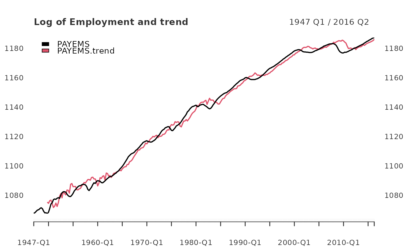
data(PAYEMS)
log_Employment <- 100*log(xts::to.quarterly(PAYEMS["1947/2016-6"], OHLC = FALSE))
employ_trend <- yth_filter(log_Employment, h = 8, p = 4, output = c("x", "trend"))
plot(employ_trend, grid.col = "white", legend.loc = "topleft",
main = "Log of Employment and trend")
 #----------------------------------------------------------------------------#
quarterly_data <- 100*log(merge(GDPC1, PCECC96, GPDIC1, EXPGSC1, IMPGSC1, GCEC1, GDPDEF))
cycle <- do.call(merge, lapply(quarterly_data, yth_filter, output = "cycle"))
random <- do.call(merge, lapply(quarterly_data, yth_filter, output = "random"))
cycle.sd <- t(data.frame(lapply(cycle, sd, na.rm = TRUE)))
GDP.cor <- t(data.frame(lapply(cycle, cor, cycle[,1], use = "complete.obs")))
random.sd <- t(data.frame(lapply(random, sd, na.rm = TRUE)))
random.cor <- t(data.frame(lapply(random, cor, random[,1], use = "complete.obs")))
my_table_2 <- round(data.frame(cbind(cycle.sd, GDP.cor, random.sd, random.cor)), 2)
names(my_table_2) <- names(Hamilton_table_2)[1:4]
my_table_2
#> cycle.sd gdp.cor random.sd gdp.rand.cor
#> GDPC1.cycle 3.27 1.00 3.55 1.00
#> PCECC96.cycle 2.90 0.80 3.08 0.82
#> GPDIC1.cycle 12.47 0.82 12.98 0.78
#> EXPGSC1.cycle 10.81 0.36 11.35 0.36
#> IMPGSC1.cycle 9.55 0.76 9.88 0.76
#> GCEC1.cycle 6.89 0.30 8.13 0.35
#> GDPDEF.cycle 3.05 0.07 4.04 -0.09
#----------------------------------------------------------------------------#
quarterly_data <- 100*log(merge(GDPC1, PCECC96, GPDIC1, EXPGSC1, IMPGSC1, GCEC1, GDPDEF))
cycle <- do.call(merge, lapply(quarterly_data, yth_filter, output = "cycle"))
random <- do.call(merge, lapply(quarterly_data, yth_filter, output = "random"))
cycle.sd <- t(data.frame(lapply(cycle, sd, na.rm = TRUE)))
GDP.cor <- t(data.frame(lapply(cycle, cor, cycle[,1], use = "complete.obs")))
random.sd <- t(data.frame(lapply(random, sd, na.rm = TRUE)))
random.cor <- t(data.frame(lapply(random, cor, random[,1], use = "complete.obs")))
my_table_2 <- round(data.frame(cbind(cycle.sd, GDP.cor, random.sd, random.cor)), 2)
names(my_table_2) <- names(Hamilton_table_2)[1:4]
my_table_2
#> cycle.sd gdp.cor random.sd gdp.rand.cor
#> GDPC1.cycle 3.27 1.00 3.55 1.00
#> PCECC96.cycle 2.90 0.80 3.08 0.82
#> GPDIC1.cycle 12.47 0.82 12.98 0.78
#> EXPGSC1.cycle 10.81 0.36 11.35 0.36
#> IMPGSC1.cycle 9.55 0.76 9.88 0.76
#> GCEC1.cycle 6.89 0.30 8.13 0.35
#> GDPDEF.cycle 3.05 0.07 4.04 -0.09