Fits Hamilton's alternative model

yth_glm fits a generalized linear model suggested by James D. Hamilton as a better alternative to the Hodrick-Prescott Filter.

yth_glm(x, h = 8, p = 4, ...)

Arguments

x	A univariate xts object of any zoo index class, such as Date, yearmon, or yearqtr. For converting objects of type timeSeries, ts, irts, fts, matrix, data.frame or zoo to xts, please read as.xts.
h	An integer, defining the lookahead period. Defaults to h = 8, suggested by Hamilton. The default assumes economic data of quarterly periodicity with a lookahead period of 2 years. This function is not limited by the default parameter, and Econometricians may change it as required.
p	An integer, indicating the number of lags. A Default of p = 4, suggested by Hamilton, assumes data is of quarterly periodicity. If data is of monthly periodicity, one may choose p = 12 or aggregate the series to quarterly periodicity and maintain the default. Econometricians should use this parameter to accommodate the Seasonality of their data.
...	all arguments passed to the function glm

Value

yth_glm returns a generalized linear model object of class glm, which inherits from lm.

Details

For time series of quarterly periodicity, Hamilton suggests parameters of h = 8 and p = 4, or an \(AR(4)\) process, additionally lagged by \(8\) lookahead periods. Econometricians may explore variations of h. However, p is designed to correspond with the seasonality of a given periodicity and should be matched accordingly. $$y_{t+h} = \beta_0 + \beta_1 y_t + \beta_2 y_{t-1} + \beta_3 y_{t-2} + \beta_4 y_{t-3} + v_{t+h}$$ $$\hat{v}_{t+h} = y_{t+h} - \hat{\beta}_0 + \hat{\beta}_1 y_t + \hat{\beta}_2 y_{t-1} + \hat{\beta}_3 y_{t-2} + \hat{\beta}_4 y_{t-3}$$ Which can be rewritten as: $$y_{t} = \beta_0 + \beta_1 y_{t-8} + \beta_2 y_{t-9} + \beta_3 y_{t-10} + \beta_4 y_{t-11} + v_{t}$$ $$\hat{v}_{t} = y_{t} - \hat{\beta}_0 + \hat{\beta}_1 y_{t-8} + \hat{\beta}_2 y_{t-9} + \hat{\beta}_3 y_{t-10} + \hat{\beta}_4 y_{t-11}$$

References

James D. Hamilton. Why You Should Never Use the Hodrick-Prescott Filter. NBER Working Paper No. 23429, Issued in May 2017.

See also

glm

Examples

data(GDPC1)

gdp_model <- yth_glm(GDPC1, h = 8, p = 4, family = gaussian)

summary(gdp_model)
#> 
#> Call:
#> stats::glm(formula = formula, family = ..1, data = data)
#> 
#> Deviance Residuals: 
#>      Min        1Q    Median        3Q       Max  
#> -2092.34   -165.56     37.48    197.80    640.61  
#> 
#> Coefficients:
#>             Estimate Std. Error t value Pr(>|t|)    
#> (Intercept) 224.3629    37.8312   5.931 8.84e-09 ***
#> xt_0          1.6942     0.3096   5.472 9.87e-08 ***
#> xt_1         -0.5404     0.5041  -1.072    0.285    
#> xt_2         -0.3198     0.5050  -0.633    0.527    
#> xt_3          0.1898     0.3113   0.610    0.543    
#> ---
#> Signif. codes:  0 ‘***’ 0.001 ‘**’ 0.01 ‘*’ 0.05 ‘.’ 0.1 ‘ ’ 1
#> 
#> (Dispersion parameter for gaussian family taken to be 99574.7)
#> 
#>     Null deviance: 7702056096  on 285  degrees of freedom
#> Residual deviance:   27980490  on 281  degrees of freedom
#>   (11 observations deleted due to missingness)
#> AIC: 4110.1
#> 
#> Number of Fisher Scoring iterations: 2
#> 

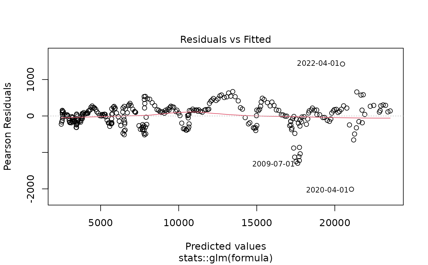
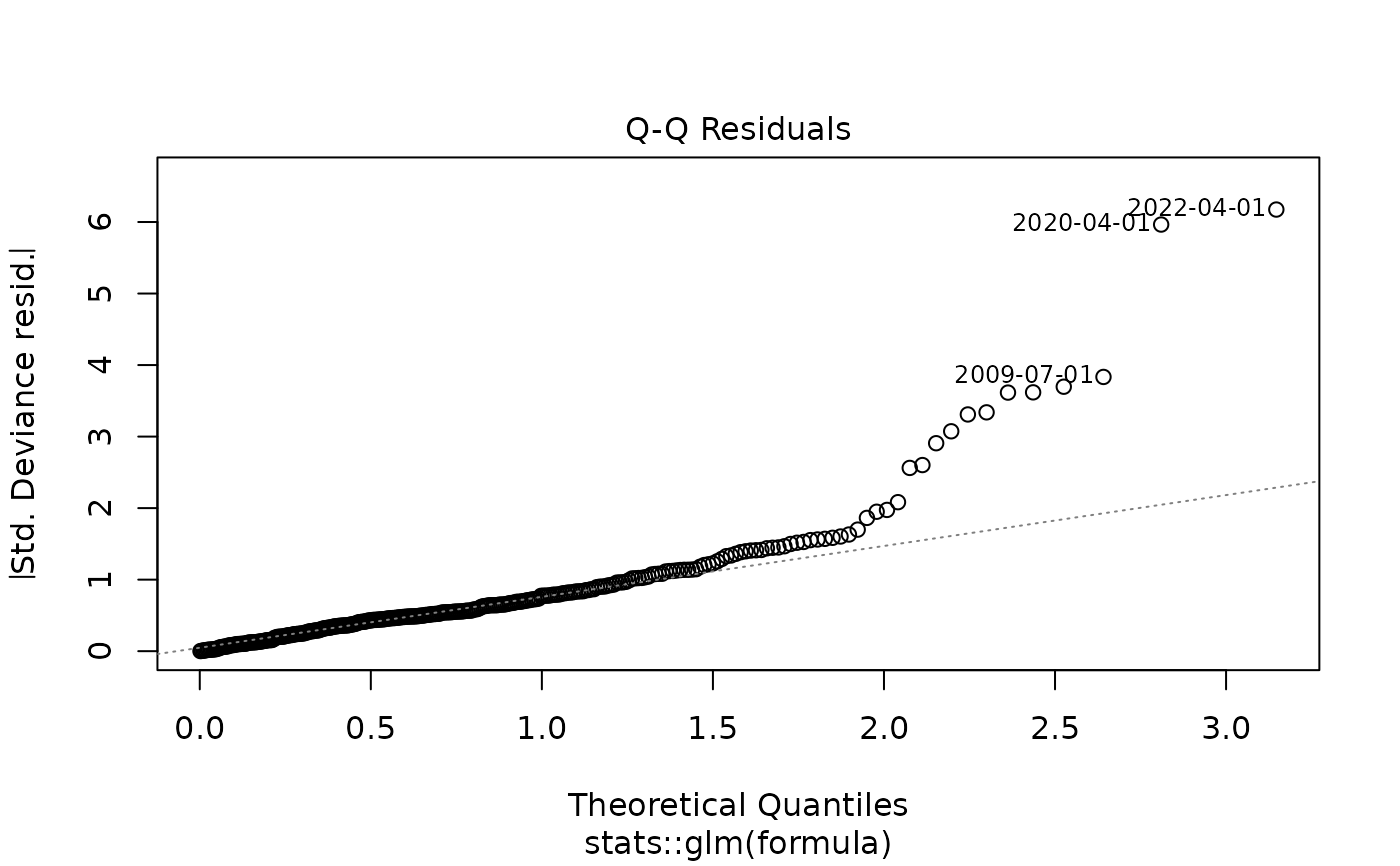
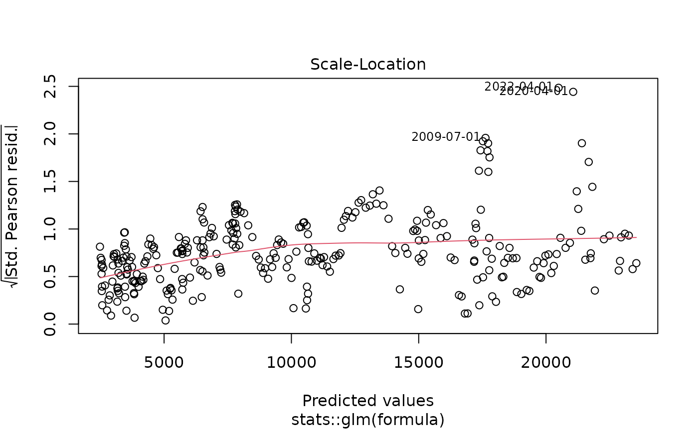
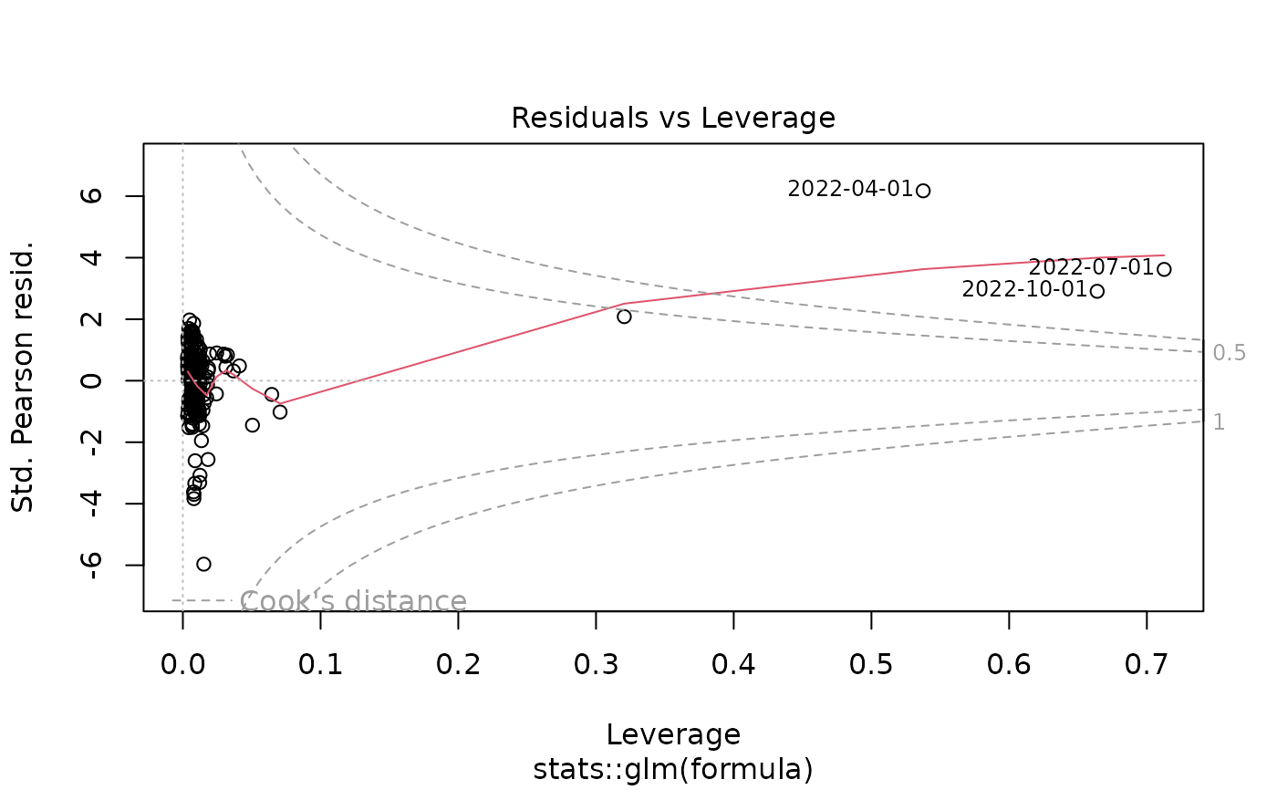
plot(gdp_model)