Reproducing Hamilton

In the working paper titled “Why You Should Never Use the Hodrick-Prescott Filter”, James D. Hamilton proposes an interesting new alternative to economic time series filtering. The neverhpfilter package provides functions for implementing his solution. Hamilton (2017) <doi:10.3386/w23429>

Hamilton’s abstract offers an excellent introduction to the problem and alternative solution:

The HP filter produces series with spurious dynamic relations that have no basis in the underlying data-generating process.

Filtered values at the end of the sample are very different from those in the middle, and are also characterized by spurious dynamics.

A statistical formalization of the problem typically produces values for the smoothing parameter vastly at odds with common practice, e.g., a value for $\lambda$ far below 1600 for quarterly data.

There’s a better alternative. A regression of the variable at date $t + h$ on the four most recent values as of date $t$ offers a robust approach to detrending that achieves all the objectives sought by users of the HP filter with none of its drawbacks.

Using quarterly economic data, Hamilton suggests a linear model on a univariate time series shifted ahead by h periods, regressed against a series of variables constructed from varying lags of the series by some number of periods, p. A modified auto-regressive $AR(p)$ model, dependent on a $t+h$ look-ahead, if you will. This is expressed more specifically by:

$y_{t+8} = \beta_0 + \beta_1 y_t + \beta_2 y_{t-1} +\beta_3 y_{t-2} + \beta_4 y_{t-3} + v_{t+8}$ $\hat{v}_{t+8} = y_{t+8} + \hat{\beta}_0 + \hat{\beta}_1 y_t + \hat{\beta}_2 y_{t-1} + \hat{\beta}_3 y_{t-2} + \hat{\beta}_4 y_{t-3}$

Which can be rewritten as:

$y_{t} = \beta_0 + \beta_1 y_{t-8} + \beta_2 y_{t-9} + \beta_3 y_{t-10} + \beta_4 y_{t-11} + v_{t}$

$\hat{v}_{t} = y_{t} - \hat{\beta}_0 + \hat{\beta}_1 y_{t-8} + \hat{\beta}_2 y_{t-9} + \hat{\beta}_3 y_{t-10} + \hat{\beta}_4 y_{t-11}$

Implementation

First, lets run the yth_filter on Real GDP using the default settings suggested by Hamilton of an $h = 8$ look-ahead period (2 years) and $p = 4$ lags (1 year). The output is displayed below containing the original series, trend, cycle, and random components.

The random component is simply the difference between the original series and its $h$ look ahead, which is why it leads 8 NA observations. Due to the $h$ and $p$ parameters, trend and cycle components lead with 11 NA observations.

library(neverhpfilter)

data(GDPC1)

gdp_filter <- yth_filter(100*log(GDPC1), h = 8, p = 4)

head(data.frame(Date=index(gdp_filter), coredata(gdp_filter)), 15)

##          Date    GDPC1 GDPC1.trend GDPC1.cycle GDPC1.random
## 1  1947-01-01 768.8309          NA          NA           NA
## 2  1947-04-01 768.5653          NA          NA           NA
## 3  1947-07-01 768.3603          NA          NA           NA
## 4  1947-10-01 769.9141          NA          NA           NA
## 5  1948-01-01 771.4089          NA          NA           NA
## 6  1948-04-01 773.0478          NA          NA           NA
## 7  1948-07-01 773.6207          NA          NA           NA
## 8  1948-10-01 773.7339          NA          NA           NA
## 9  1949-01-01 772.3477          NA          NA     3.516789
## 10 1949-04-01 772.0075          NA          NA     3.442130
## 11 1949-07-01 773.0361          NA          NA     4.675851
## 12 1949-10-01 772.1948    779.1321  -6.9373485     2.280665
## 13 1950-01-01 776.0511    780.3038  -4.2526309     4.642219
## 14 1950-04-01 779.0565    781.5229  -2.4664958     6.008660
## 15 1950-07-01 782.8487    782.1703   0.6783457     9.228028

Comparing our estimates with Hamilton’s

In this next section, I reproduce a few of Hamilton’s tables and graphs, to make sure the functions approximately match his results.

In the Appendix, Employment (All Employees: Total Non-farm series) is plotted in the form of $100 * log($ PAYEMS $)$ and superimposed with it’s random walk representation. (Hamilton 44). There are many good reasons to use xts when handling time series data. Two of them are illustrated below in efficiently transforming monthly series to.quarterly and in ploting the results of yth_filter.

data(PAYEMS)
log_Employment <- 100*log(xts::to.quarterly(PAYEMS["1947/2016-6"], OHLC = FALSE))

employ_trend <- yth_filter(log_Employment, h = 8, p = 4, output = c("x", "trend"), family = gaussian)

plot.xts(employ_trend, grid.col = "white", legend.loc = "topleft", main = "Log of Employment and trend")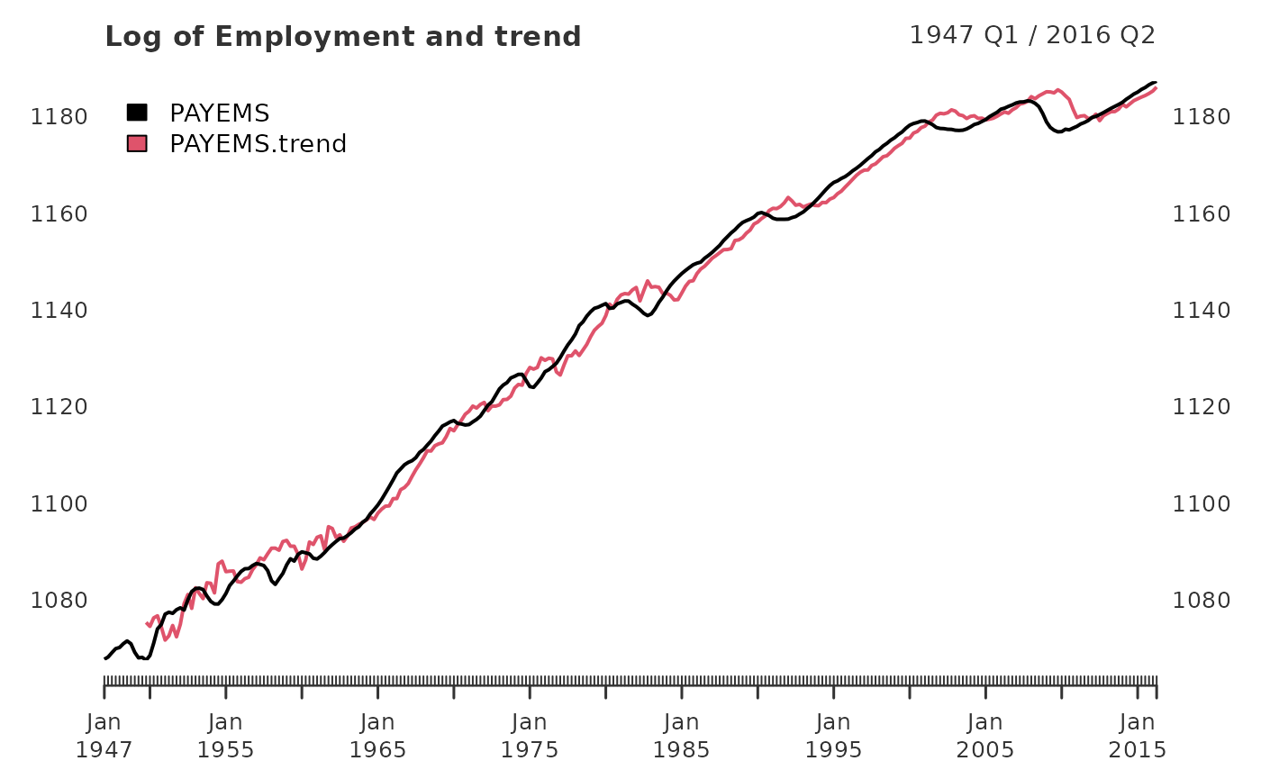

When filtering time series, the cycle component is of great interest. Here, it is graphed alongside a random walk representation (Hamilton 44).

employ_cycle <- yth_filter(log_Employment, h = 8, p = 4, output = c("cycle", "random"), family = gaussian)

plot.xts(employ_cycle, grid.col = "white", legend.loc = "topright", main="Log of Employment cycle and random")
abline(h=0)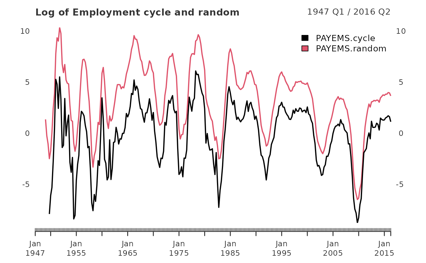

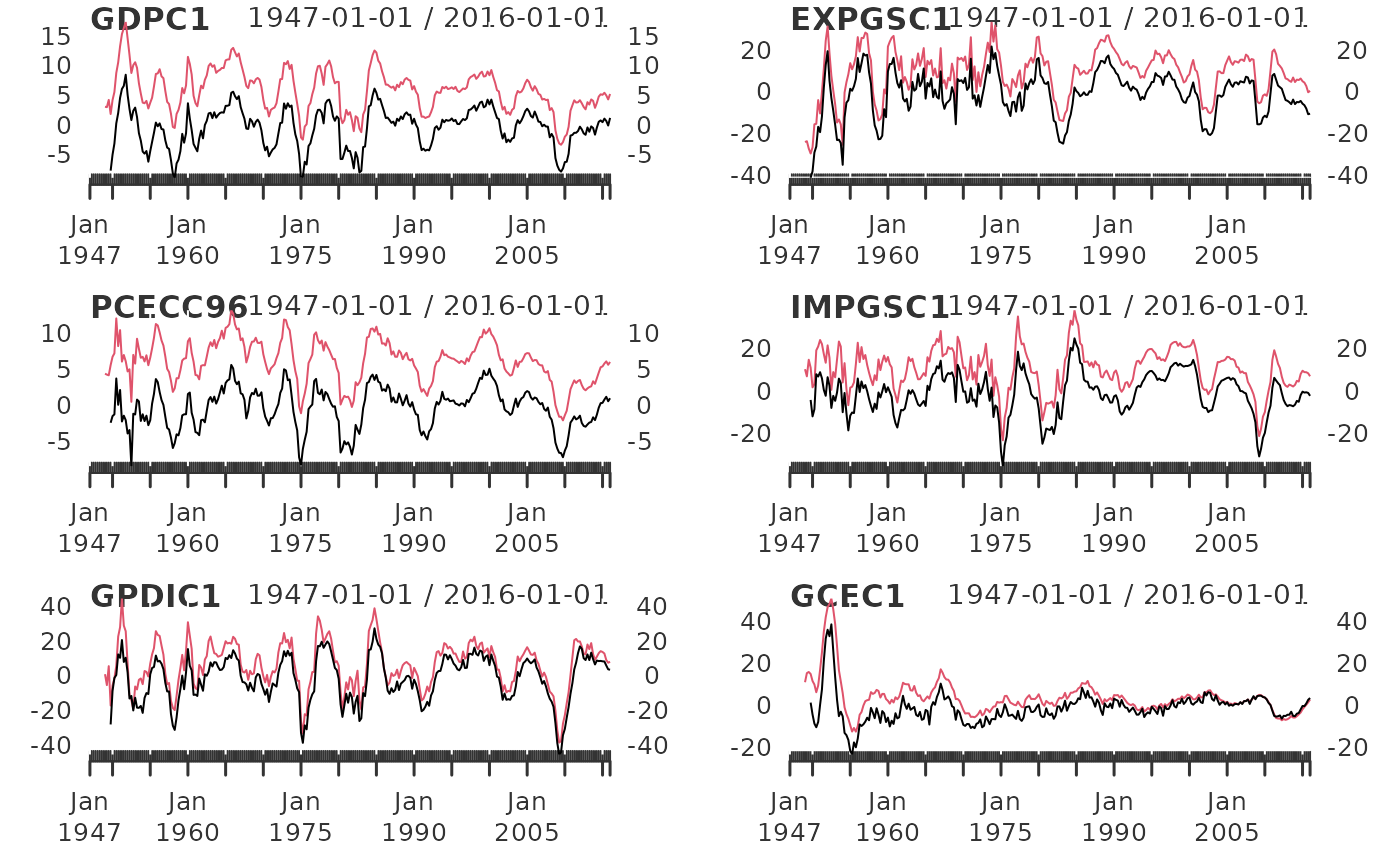
Turning the page, we find a similar graph of the cyclical component of $100 * log$ of GDP, Exports, Consumption, Imports, Investment, and Government (Hamilton 45).

Below I merge these data into one xts object and write a function wrapper around yth_filter and plot, which is then lapply’d over each series, producing a plot for each one.

fig6_data <- 100*log(merge(GDPC1, EXPGSC1, PCECC96, IMPGSC1, GPDIC1, GCEC1)["1947/2016-3"])

fig6_wrapper <- function(x, ...) {
               cycle <-  yth_filter(x, h = 8, p = 4, output = c("cycle", "random"), family = gaussian)
               plot.xts(cycle, grid.col = "white", lwd=1, main = names(x))
}

par(mfrow=c(3,2))
lapply(fig6_data, fig6_wrapper)

When striving to recreate a statistical method found in a journal or paper, one can perform surprisingly well by thoroughly digesting the relevant sections and “eyeballing” graphs included in the original author’s work.

Better still, is finding a table presenting said author’s estimates, which one can use to directly compare with their own. Fortunately for us, Hamilton’s Appendix displays such a table which I use here to test against functions contained in neverhpfilter.

His results are displayed below in table 2 (Hamilton 40), which I’ve stored as a data.frame in this package.

data("Hamilton_table_2")
?Hamilton_table_2

Hamilton_table_2[-NROW(Hamilton_table_2),]

##                        cycle.sd gdp.cor random.sd gdp.rand.cor        Sample
## GDP                        3.38    1.00      3.69         1.00 1947-1/2016-1
## Consumption                2.85    0.79      3.04         0.82 1947-1/2016-1
## Investment                13.19    0.84     13.74         0.80 1947-1/2016-1
## Exports                   10.77    0.33     11.33         0.30 1947-1/2016-1
## Imports                    9.79    0.77      9.98         0.75 1947-1/2016-1
## Government-spending        7.13    0.31      8.60         0.38 1947-1/2016-1
## Employment                 3.09    0.85      3.32         0.85 1947-1/2016-2
## Unemployment-rate          1.44   -0.81      1.72        -0.79 1948-1/2016-2
## GDP-Deflator               2.99    0.04      4.11        -0.13 1947-1/2016-1
## S&P500                    21.80    0.41     22.08         0.38 1950-1/2016-2
## 10-year-Treasury-yield     1.46   -0.05      1.51         0.08 1953-2/2016-2
## Fedfunds-rate              2.78    0.33      3.03         0.40 1954-3/2016-2

I’ll replicate the table above, combining base R functions with estimates of the yth_filter function.

The first step is to combine our economic time series into an object that allows for convenient iteration of computations across all data of interest. First, merge all series of quarterly frequency. These are GDPC1, PCECC96, GPDIC1, EXPGSC1, IMPGSC1, GCEC1, GDPDEF. At this point, subset observations by the precise date range used by Hamilton. At some point, all series which are measured in prices need to be given the $100*log$ treatment, so do this now.

quarterly_data <- 100*log(merge(GDPC1, PCECC96, GPDIC1, EXPGSC1, IMPGSC1, GCEC1, GDPDEF)["1947/2016-3"])

Some economic time series we wish to compare are measured in monthly periodicity, so we need to lower their frequency to.quarterly. merge monthly series and $100*log$ those expressed in prices. Leave data measured in percentages be. Then, functionally iterate over every series and transform them to.quarterly. Finally, all series are combined into one xts object, I call quarterly_data.

monthly_data <- merge(100*log(PAYEMS), 100*log(SP500$SP500)["1950/"], UNRATENSA, GS10, FEDFUNDS)

to_quarterly_data <- do.call(merge, lapply(monthly_data, to.quarterly, OHLC = FALSE))["1947/2016-6"]

quarterly_data <- merge(quarterly_data, to_quarterly_data)

Now its time to functionally iterate over each series. I do this by lapplying the yth_filter to each series, while iteratively mergeing results into one object with do.call. The optional argument of output = "cycle" is convenient here as it returns the labeled univariate cycle component for each series. For example, GDPCE1.cycle. The same approach is use to compute the random component for each series as well.

cycle <- do.call(merge, lapply(quarterly_data, yth_filter, output = "cycle"))

random <- do.call(merge, lapply(quarterly_data, yth_filter, output = "random"))

Now that all data have been transformed into both cycle and random series, its time to estimate the standard deviation for each, as well as each components correlation with GDP. This is also a good opportunity to transpose each of our estimates into vertical columned data.frames, matching Hamilton’s format.

cycle.sd <- t(data.frame(lapply(cycle, sd, na.rm = TRUE)))
GDP.cor <- t(data.frame(lapply(cycle, cor, cycle[,1], use = "complete.obs")))
random.sd <- t(data.frame(lapply(random, sd, na.rm = TRUE)))
random.cor <- t(data.frame(lapply(random, cor, random[,1], use = "complete.obs")))

my_table_2 <- round(data.frame(cbind(cycle.sd, GDP.cor, random.sd, random.cor)), 2)

Hamilton displays the date ranges of his samples, so we will do the same, while keeping the xts date range syntax format. I use a simple function I call sample_range to extract the first and last observation of each series’ index.xts. This approach serves as a check on the work, as oppose to manually creating labels. Sample ranges are then transposed into vertical data.frames and cbind’d to the existing table of estimates.

sample_range <- function(x) {
  x <- na.omit(x)
  gsub(" ", "-", paste0(index(x[1,]), "/", index(x[NROW(x),])))
}

data_sample <- t(data.frame(lapply(quarterly_data, sample_range)))

my_table_2 <- cbind(my_table_2, data_sample)
names(my_table_2) <- names(Hamilton_table_2)

Finally, rbind Hamilton’s table 2 with my table for a visual comparison. The results are nearly identical, inspiring confidence in the replication of the approach, as the functions of the neverhpfilter package.

According to the ‘code and data’ link on the ‘Current Working Papers’ page of Hamilton’s site, both Matlab and RATS were used for computation of the table. It is not surprising that minor differences in estimates would occur, likely due to differences in the underlying data or internal computational choices made by each commercial software product. While economic time series are publicly available and have a central source at FRED, that is not so for Standard & Poor’s index data. Unsurprisingly, the SP500 data shows the most divergence, and it is not clear what source was used in the original paper (though I have my suspicions for future exploration).

Below, see Hamilton’s table 2 compared with estimates from neverhpfilter::yth_filter, sorted by standard deviation of the cycle component. yth_filter estimates are labeled with the suffix .cycle

 # Combined table
combined_table <- rbind(Hamilton_table_2[-NROW(Hamilton_table_2),], my_table_2)

combined_table[order(combined_table$cycle.sd),]

##                        cycle.sd gdp.cor random.sd gdp.rand.cor
## Unemployment-rate          1.44   -0.81      1.72        -0.79
## UNRATENSA.cycle            1.44   -0.82      1.71        -0.80
## 10-year-Treasury-yield     1.46   -0.05      1.51         0.08
## GS10.cycle                 1.46   -0.05      1.51         0.08
## Fedfunds-rate              2.78    0.33      3.03         0.40
## FEDFUNDS.cycle             2.78    0.33      3.03         0.41
## PCECC96.cycle              2.82    0.78      3.00         0.82
## Consumption                2.85    0.79      3.04         0.82
## GDP-Deflator               2.99    0.04      4.11        -0.13
## GDPDEF.cycle               3.01    0.03      4.13        -0.14
## Employment                 3.09    0.85      3.32         0.85
## PAYEMS.cycle               3.09    0.85      3.32         0.85
## GDPC1.cycle                3.35    1.00      3.63         1.00
## GDP                        3.38    1.00      3.69         1.00
## Government-spending        7.13    0.31      8.60         0.38
## GCEC1.cycle                7.16    0.32      8.59         0.38
## IMPGSC1.cycle              9.71    0.76      9.87         0.75
## Imports                    9.79    0.77      9.98         0.75
## EXPGSC1.cycle             10.75    0.33     11.33         0.30
## Exports                   10.77    0.33     11.33         0.30
## GPDIC1.cycle              13.18    0.83     13.67         0.78
## Investment                13.19    0.84     13.74         0.80
## SP500.cycle               21.38    0.42     21.60         0.40
## S&P500                    21.80    0.41     22.08         0.38
##                                       Sample
## Unemployment-rate              1948-1/2016-2
## UNRATENSA.cycle        1948-01-01/2016-04-01
## 10-year-Treasury-yield         1953-2/2016-2
## GS10.cycle             1953-04-01/2016-04-01
## Fedfunds-rate                  1954-3/2016-2
## FEDFUNDS.cycle         1954-07-01/2016-04-01
## PCECC96.cycle          1947-01-01/2016-01-01
## Consumption                    1947-1/2016-1
## GDP-Deflator                   1947-1/2016-1
## GDPDEF.cycle           1947-01-01/2016-01-01
## Employment                     1947-1/2016-2
## PAYEMS.cycle           1947-01-01/2016-04-01
## GDPC1.cycle            1947-01-01/2016-01-01
## GDP                            1947-1/2016-1
## Government-spending            1947-1/2016-1
## GCEC1.cycle            1947-01-01/2016-01-01
## IMPGSC1.cycle          1947-01-01/2016-01-01
## Imports                        1947-1/2016-1
## EXPGSC1.cycle          1947-01-01/2016-01-01
## Exports                        1947-1/2016-1
## GPDIC1.cycle           1947-01-01/2016-01-01
## Investment                     1947-1/2016-1
## SP500.cycle            1950-01-01/2016-04-01
## S&P500                         1950-1/2016-2

Summary

The estimates generated with the neverhpfilter package are nearly identical to those displayed by Hamilton (2017). If one has the use case, the generalized functions which inherit methods from glm and xts will estimate higher frequency time series as well as error distributions other than Gaussian. In addition to consulting the paper which inspired this package, check out the documentation for yth_filter to learn more, or reach out to me with any questions.

Justin M Shea

Implementation

Comparing our estimates with Hamilton’s

Summary