Introductory Econometrics Examples

Justin M Shea

Introduction

This vignette reproduces examples from various chapters of Introductory Econometrics: A Modern Approach, 7e by Jeffrey M. Wooldridge. Each example illustrates how to load data, build econometric models, and compute estimates with R.

In addition, the Appendix cites a few sources using R for econometrics. Of note, in 2020 Florian Heiss published a 2nd edition of Using R for Introductory Econometrics; it is excellent. The Heiss text is a companion to wooldridge for R users, and offers an in depth treatment with several worked examples from each chapter. Indeed, his example use this wooldridge package as well.

Now, install and load the wooldridge package and lets get started!

install.packages("wooldridge")

library(wooldridge)

Chapter 2: The Simple Regression Model

Example 2.10: A Log Wage Equation

Load the wage1 data and check out the documentation.

data("wage1")

?wage1

The documentation indicates these are data from the 1976 Current Population Survey, collected by Henry Farber when he and Wooldridge were colleagues at MIT in 1988.

$educ$: years of education

$wage$: average hourly earnings

$lwage$: log of the average hourly earnings

First, make a scatter-plot of the two variables and look for possible patterns in the relationship between them.

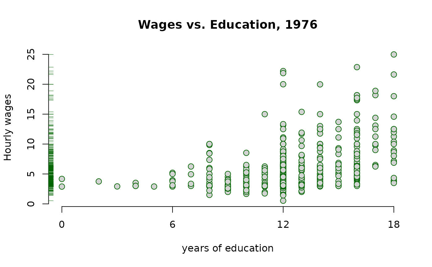
It appears that on average, more years of education, leads to higher wages.

The example in the text is interested in the return to another year of education, or what the percentage change in wages one might expect for each additional year of education. To do so, one must use the $log($wage$)$. This has already been computed in the data set and is defined as lwage.

The textbook provides excellent discussions around these topics, so please consult it.

Build a linear model to estimate the relationship between the log of wage (lwage) and education (educ).

$$\widehat{log(wage)} = \beta_0 + \beta_1educ$$

log_wage_model <- lm(lwage ~ educ, data = wage1)

Print the summary of the results.

summary(log_wage_model)

	Dependent variable:
	lwage
educ	0.08274*** (0.00757)
Constant	0.58377*** (0.09734)
Observations	526
R2	0.18581
Adjusted R2	0.18425
Residual Std. Error	0.48008 (df = 524)
F Statistic	119.58160*** (df = 1; 524)
Note:	p<0.1; p<0.05; p<0.01

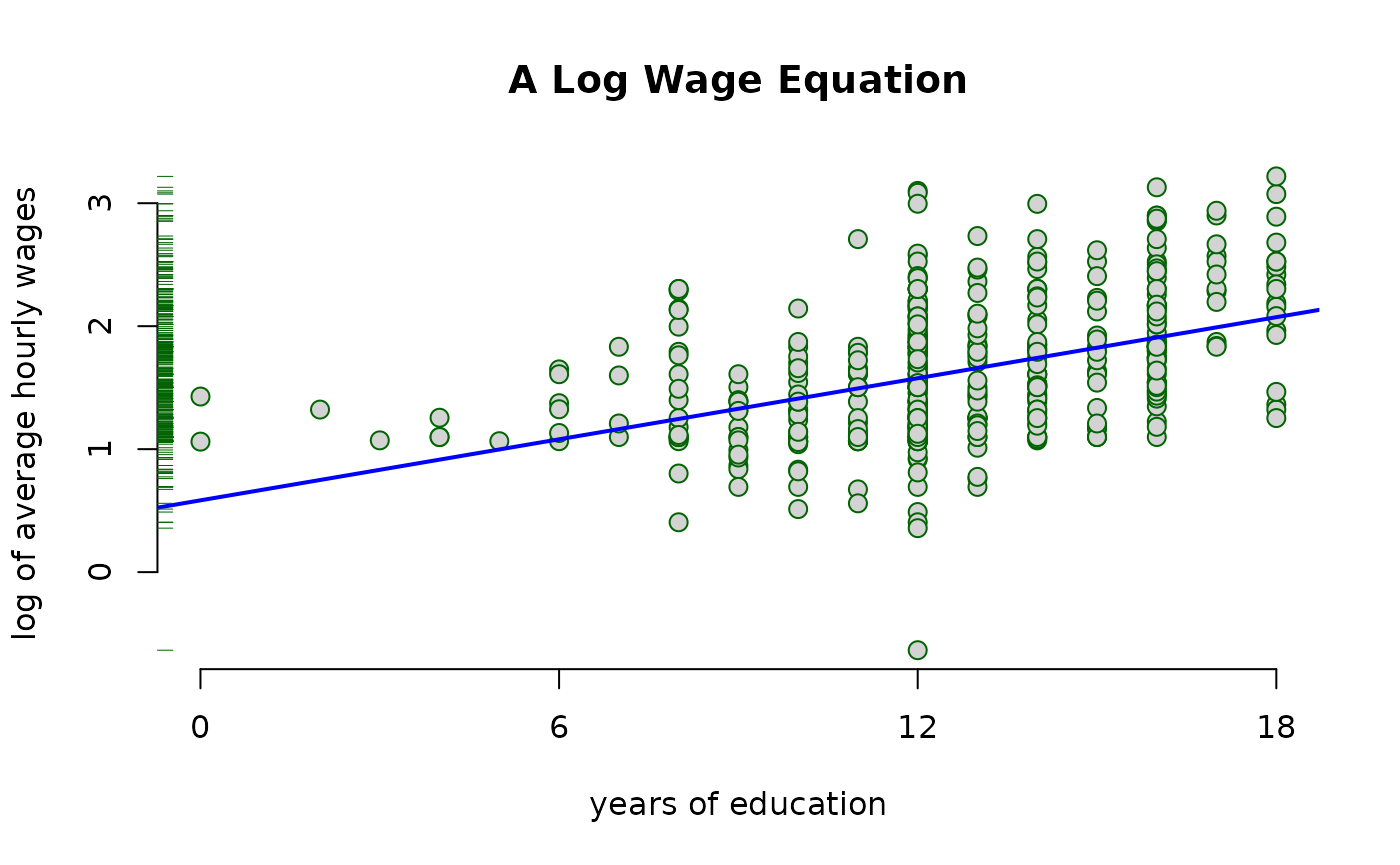
Plot the $log($wage$)$ vs educ. The blue line represents the least squares fit.

Chapter 3: Multiple Regression Analysis: Estimation

Example 3.2: Hourly Wage Equation

Check the documentation for variable information

?wage1

$lwage$: log of the average hourly earnings

$educ$: years of education

$exper$: years of potential experience

$tenutre$: years with current employer

Plot the variables against lwage and compare their distributions and slope ($\beta$) of the simple regression lines.

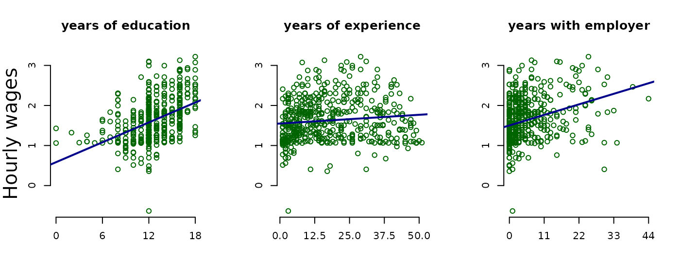
Estimate the model regressing educ, exper, and tenure against log(wage).

$$\widehat{log(wage)} = \beta_0 + \beta_1educ + \beta_3exper + \beta_4tenure$$

hourly_wage_model <- lm(lwage ~ educ + exper + tenure, data = wage1)

Print the estimated model coefficients:

coefficients(hourly_wage_model)

	Coefficients
(Intercept)	0.2844
educ	0.0920
exper	0.0041
tenure	0.0221

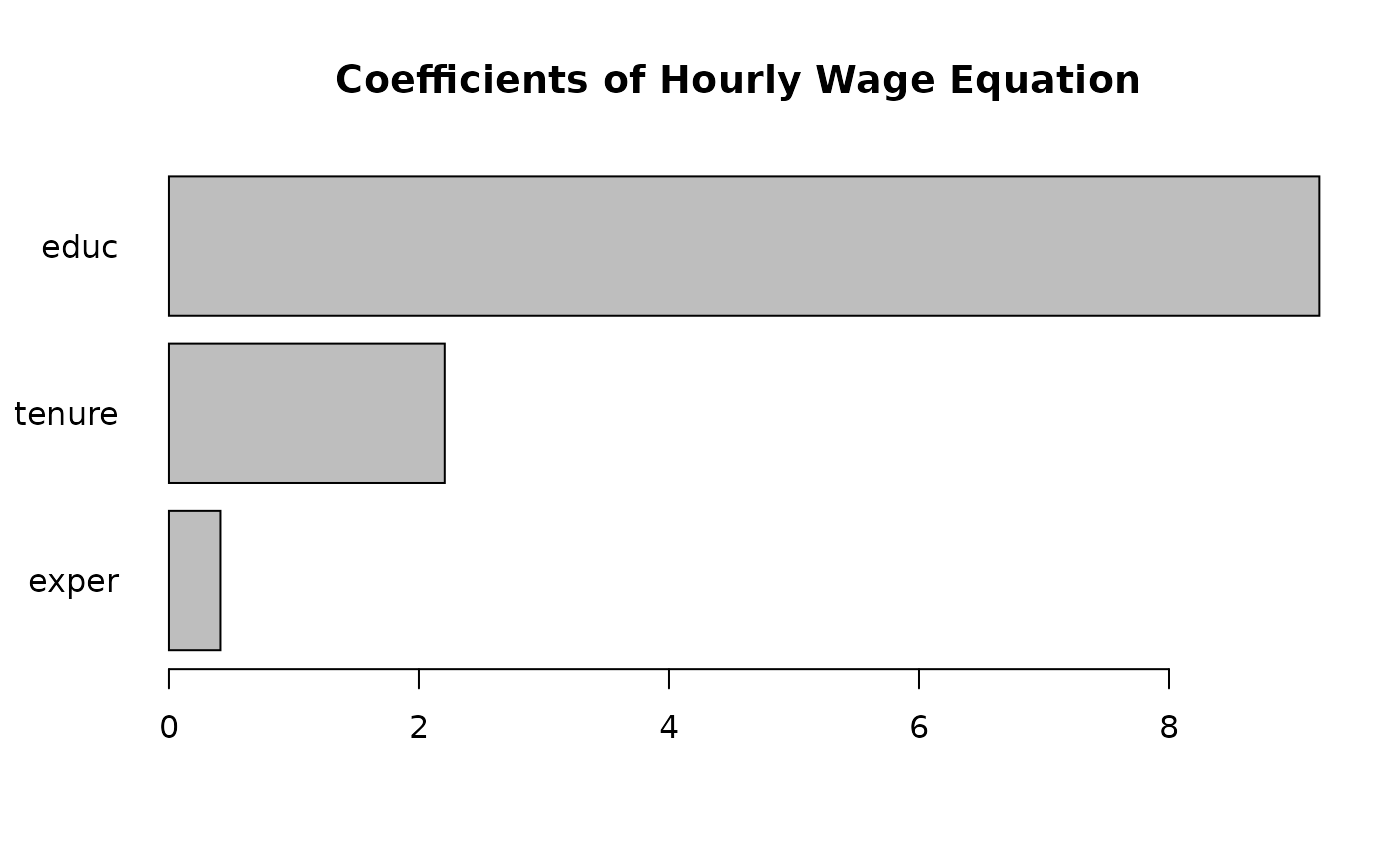
Plot the coefficients, representing percentage impact of each variable on $log($wage$)$ for a quick comparison.

Chapter 4: Multiple Regression Analysis: Inference

Example 4.1 Hourly Wage Equation

Using the same model estimated in example: 3.2, examine and compare the standard errors associated with each coefficient. Like the textbook, these are contained in parenthesis next to each associated coefficient.

summary(hourly_wage_model)

	Dependent variable:
	lwage
educ	0.09203*** (0.00733)
exper	0.00412** (0.00172)
tenure	0.02207*** (0.00309)
Constant	0.28436*** (0.10419)
Observations	526
R2	0.31601
Adjusted R2	0.31208
Residual Std. Error	0.44086 (df = 522)
F Statistic	80.39092*** (df = 3; 522)
Note:	p<0.1; p<0.05; p<0.01

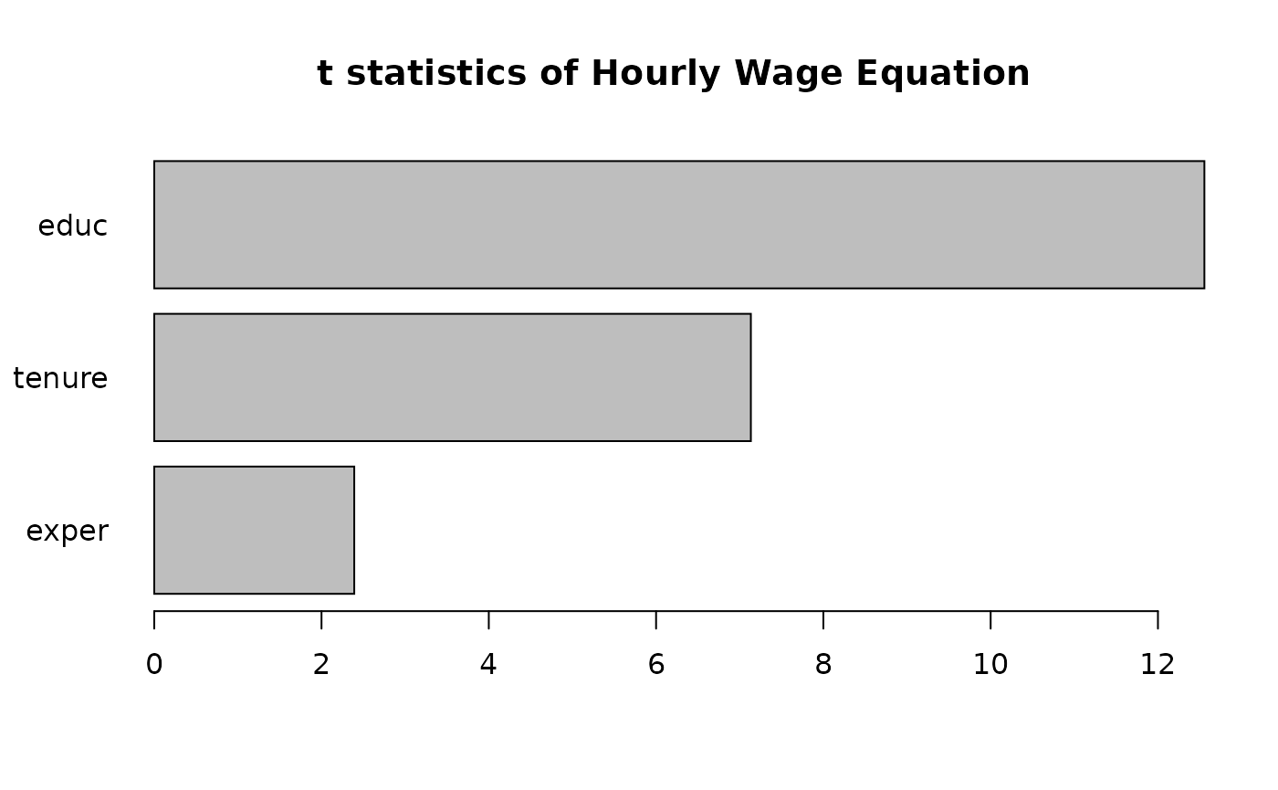
For the years of experience variable, or exper, use coefficient and Standard Error to compute the $t$ statistic:

$$t_{exper} = \frac{0.004121}{0.001723} = 2.391$$

Fortunately, R includes $t$ statistics in the summary of model diagnostics.

summary(hourly_wage_model)$coefficients

	Estimate	Std. Error	t value	Pr(>|t|)
(Intercept)	0.28436	0.10419	2.72923	0.00656
educ	0.09203	0.00733	12.55525	0.00000
exper	0.00412	0.00172	2.39144	0.01714
tenure	0.02207	0.00309	7.13307	0.00000

Plot the $t$ statistics for a visual comparison:

Example 4.7 Effect of Job Training on Firm Scrap Rates

Load the jtrain data set.

data("jtrain")

?jtrain

From H. Holzer, R. Block, M. Cheatham, and J. Knott (1993), Are Training Subsidies Effective? The Michigan Experience, Industrial and Labor Relations Review 46, 625-636. The authors kindly provided the data.

$year:$ 1987, 1988, or 1989

$union:$ =1 if unionized

$lscrap:$ Log(scrap rate per 100 items)

$hrsemp:$ (total hours training) / (total employees trained)

$lsales:$ Log(annual sales, $)

$lemploy:$ Log(umber of employees at plant)

First, use the subset function and it’s argument by the same name to return observations which occurred in 1987 and are not union. At the same time, use the select argument to return only the variables of interest for this problem.

jtrain_subset <- subset(jtrain, subset = (year == 1987 & union == 0),
                        select = c(year, union, lscrap, hrsemp, lsales, lemploy))

Next, test for missing values. One can “eyeball” these with R Studio’s View function, but a more precise approach combines the sum and is.na functions to return the total number of observations equal to NA.

sum(is.na(jtrain_subset))

## [1] 156

While R’s lm function will automatically remove missing NA values, eliminating these manually will produce more clearly proportioned graphs for exploratory analysis. Call the na.omit function to remove all missing values and assign the new data.frame object the name jtrain_clean.

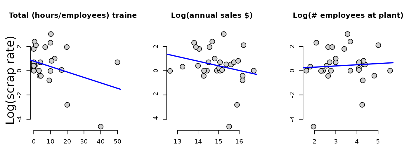
jtrain_clean <- na.omit(jtrain_subset)

Use jtrain_clean to plot the variables of interest against lscrap. Visually observe the respective distributions for each variable, and compare the slope ($\beta$) of the simple regression lines.

Now create the linear model regressing hrsemp(total hours training/total employees trained), lsales(log of annual sales), and lemploy(the log of the number of the employees), against lscrap(the log of the scrape rate).

$$lscrap = \alpha + \beta_1 hrsemp + \beta_2 lsales + \beta_3 lemploy$$

linear_model <- lm(lscrap ~ hrsemp + lsales + lemploy, data = jtrain_clean)

Finally, print the complete summary diagnostics of the model.

summary(linear_model)

	Dependent variable:
	lscrap
hrsemp	-0.02927 (0.02280)
lsales	-0.96203** (0.45252)
lemploy	0.76147* (0.40743)
Constant	12.45837** (5.68677)
Observations	29
R2	0.26243
Adjusted R2	0.17392
Residual Std. Error	1.37604 (df = 25)
F Statistic	2.96504* (df = 3; 25)
Note:	p<0.1; p<0.05; p<0.01

Chapter 5: Multiple Regression Analysis: OLS Asymptotics

Example 5.1: Housing Prices and Distance From an Incinerator

Load the hprice3 data set.

data("hprice3")

$lprice:$ Log(selling price)

$ldist:$ Log(distance from house to incinerator, feet)

$larea:$ Log(square footage of house)

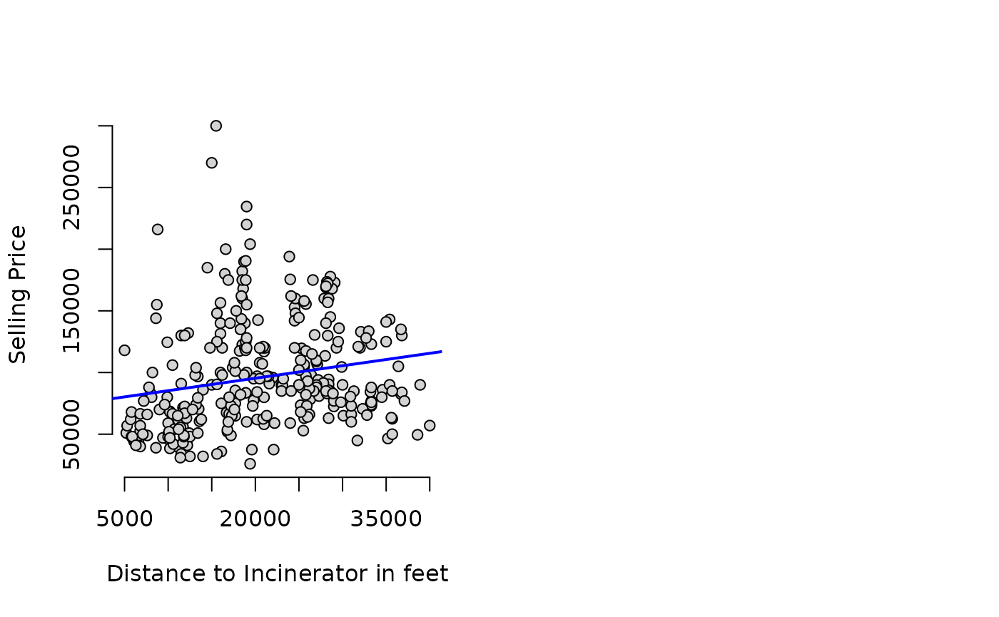
Graph the prices of housing against distance from an incinerator:

Next, model the $log($price$)$ against the $log($dist$)$ to estimate the percentage relationship between the two.

$$price = \alpha + \beta_1 dist$$

price_dist_model <- lm(lprice ~ ldist, data = hprice3)

Create another model that controls for “quality” variables, such as square footage area per house.

$$price = \alpha + \beta_1 dist + \beta_2 area$$

price_area_model <- lm(lprice ~ ldist + larea, data = hprice3)

Compare the coefficients of both models. Notice that adding area improves the quality of the model, but also reduces the coefficient size of dist.

summary(price_dist_model)
summary(price_area_model)

	Dependent variable:
	lprice
	(1)	(2)
ldist	0.31722*** (0.04811)	0.19623*** (0.03816)
larea		0.78368*** (0.05358)
Constant	8.25750*** (0.47383)	3.49394*** (0.49065)
Observations	321	321
R2	0.11994	0.47385
Adjusted R2	0.11718	0.47054
Residual Std. Error	0.41170 (df = 319)	0.31883 (df = 318)
F Statistic	43.47673*** (df = 1; 319)	143.19470*** (df = 2; 318)
Note:	p<0.1; p<0.05; p<0.01

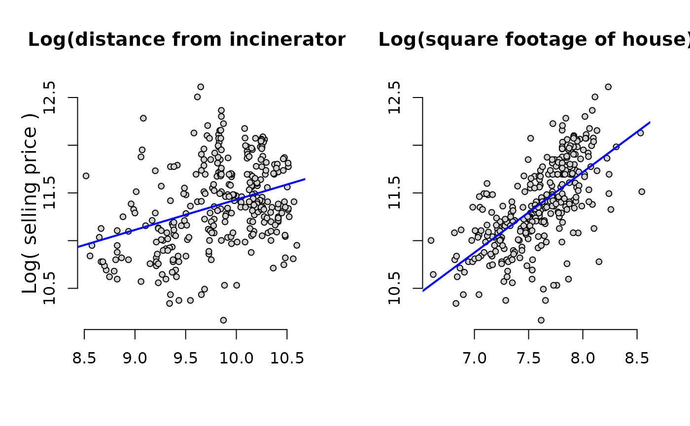
Graphing illustrates the larger coefficient for area.

Chapter 6: Multiple Regression: Further Issues

Example 6.1: Effects of Pollution on Housing Prices, standardized.

Load the hprice2 data and view the documentation.

data("hprice2")
?hprice2

Data from Hedonic Housing Prices and the Demand for Clean Air, by Harrison, D. and D.L.Rubinfeld, Journal of Environmental Economics and Management 5, 81-102. Diego Garcia, a former Ph.D. student in economics at MIT, kindly provided these data, which he obtained from the book Regression Diagnostics: Identifying Influential Data and Sources of Collinearity, by D.A. Belsey, E. Kuh, and R. Welsch, 1990. New York: Wiley.

$price$: median housing price.

$nox$: Nitrous Oxide concentration; parts per million.

$crime$: number of reported crimes per capita.

$rooms$: average number of rooms in houses in the community.

$dist$: weighted distance of the community to 5 employment centers.

$stratio$: average student-teacher ratio of schools in the community.

$$price = \beta_0 + \beta_1nox + \beta_2crime + \beta_3rooms + \beta_4dist + \beta_5stratio + \mu$$

Estimate the usual lm model.

housing_level <- lm(price ~ nox + crime + rooms + dist + stratio, data = hprice2)

Estimate the same model, but standardized coefficients by wrapping each variable with R’s scale function:

$$\widehat{zprice} = \beta_1znox + \beta_2zcrime + \beta_3zrooms + \beta_4zdist + \beta_5zstratio$$

housing_standardized <- lm(scale(price) ~ 0 + scale(nox) + scale(crime) + scale(rooms) + scale(dist) + scale(stratio), data = hprice2)

Compare results, and observe

summary(housing_level)
summary(housing_standardized)

	Dependent variable:
	price	scale(price)
	(1)	(2)
nox	-2,706.43300*** (354.08690)
crime	-153.60100*** (32.92883)
rooms	6,735.49800*** (393.60370)
dist	-1,026.80600*** (188.10790)
stratio	-1,149.20400*** (127.42870)
scale(nox)		-0.34045*** (0.04450)
scale(crime)		-0.14328*** (0.03069)
scale(rooms)		0.51389*** (0.03000)
scale(dist)		-0.23484*** (0.04298)
scale(stratio)		-0.27028*** (0.02994)
Constant	20,871.13000*** (5,054.59900)
Observations	506	506
R2	0.63567	0.63567
Adjusted R2	0.63202	0.63203
Residual Std. Error	5,586.19800 (df = 500)	0.60601 (df = 501)
F Statistic	174.47330*** (df = 5; 500)	174.82220*** (df = 5; 501)
Note:	p<0.1; p<0.05; p<0.01

Example 6.2: Effects of Pollution on Housing Prices, Quadratic Interactive Term

Modify the housing model from example 4.5, adding a quadratic term in rooms:

$$log(price) = \beta_0 + \beta_1log(nox) + \beta_2log(dist) + \beta_3rooms + \beta_4rooms^2 + \beta_5stratio + \mu$$

housing_model_4.5 <- lm(lprice ~ lnox + log(dist) + rooms + stratio, data = hprice2)

housing_model_6.2 <- lm(lprice ~ lnox + log(dist) + rooms + I(rooms^2) + stratio, 
                        data = hprice2)

Compare the results with the model from example 6.1.

summary(housing_model_4.5)
summary(housing_model_6.2)

	Dependent variable:
	lprice
	(1)	(2)
lnox	-0.95354*** (0.11674)	-0.90168*** (0.11469)
log(dist)	-0.13434*** (0.04310)	-0.08678** (0.04328)
rooms	0.25453*** (0.01853)	-0.54511*** (0.16545)
I(rooms2)		0.06226*** (0.01280)
stratio	-0.05245*** (0.00590)	-0.04759*** (0.00585)
Constant	11.08386*** (0.31811)	13.38548*** (0.56647)
Observations	506	506
R2	0.58403	0.60281
Adjusted R2	0.58071	0.59884
Residual Std. Error	0.26500 (df = 501)	0.25921 (df = 500)
F Statistic	175.85520*** (df = 4; 501)	151.77040*** (df = 5; 500)
Note:	p<0.1; p<0.05; p<0.01

Estimate the minimum turning point at which the rooms interactive term changes from negative to positive.

$$x = \frac{\hat{\beta_1}}{2\hat{\beta_2}}$$

beta_1 <- summary(housing_model_6.2)$coefficients["rooms",1] 
beta_2 <- summary(housing_model_6.2)$coefficients["I(rooms^2)",1]
turning_point <- abs(beta_1 / (2*beta_2))

print(turning_point)

## [1] 4.37763

Compute the percent change across a range of average rooms. Include the smallest, turning point, and largest.

Rooms <- c(min(hprice2$rooms), 4, turning_point, 5, 5.5, 6.45, 7.5, max(hprice2$rooms))
Percent.Change <- 100*(beta_1 + 2*beta_2*Rooms)

kable(data.frame(Rooms, Percent.Change))

Rooms	Percent.Change
3.56000	-10.181324
4.00000	-4.702338
4.37763	0.000000
5.00000	7.749903
5.50000	13.976023
6.45000	25.805651
7.50000	38.880503
8.78000	54.819367

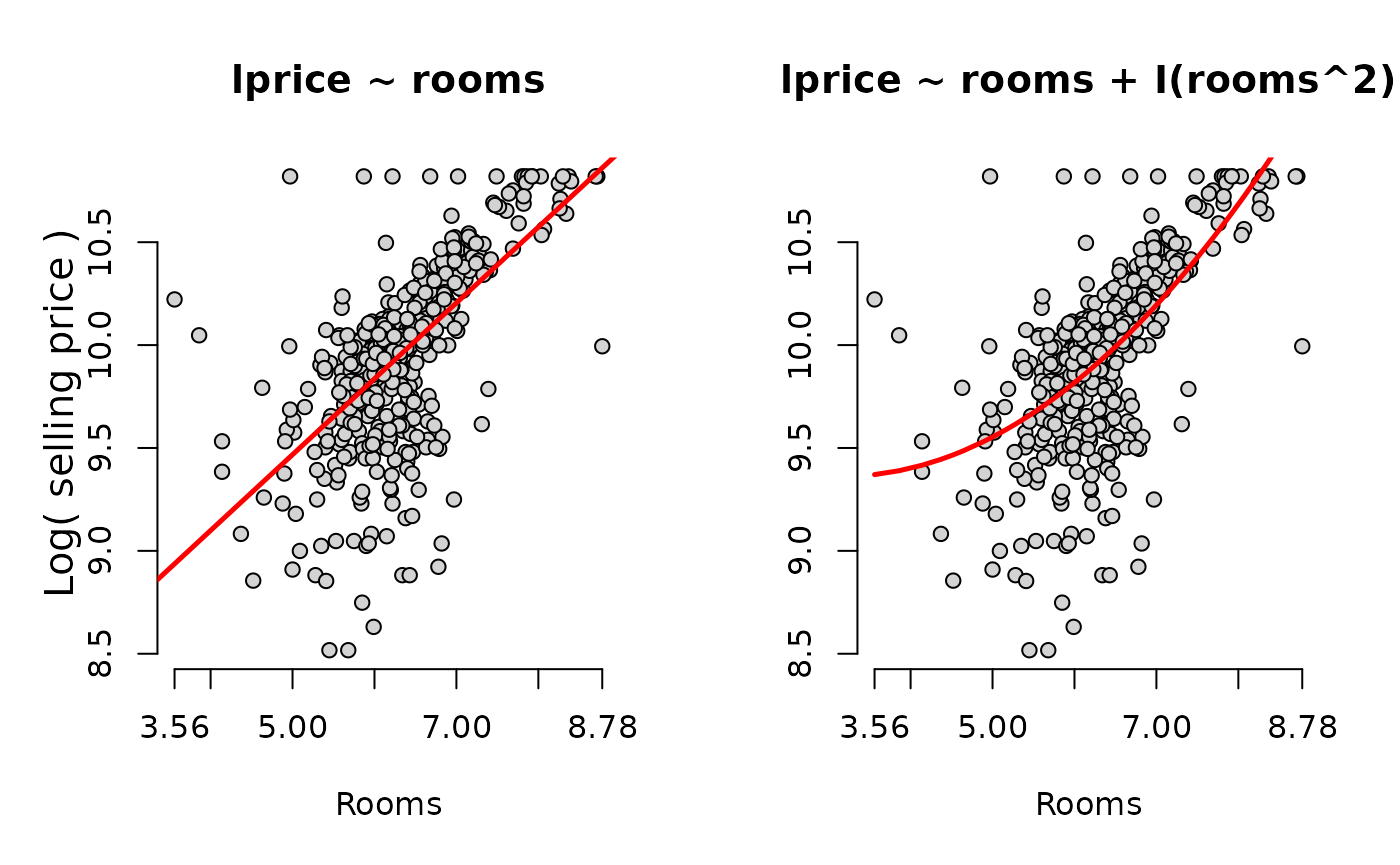
Graph the log of the selling price against the number of rooms. Superimpose a simple model as well as a quadratic model and examine the difference.

Chapter 7: Multiple Regression Analysis with Qualitative Information

Example 7.4: Housing Price Regression, Qualitative Binary variable

This time, use the hrprice1 data.

data("hprice1")

?hprice1

Data collected from the real estate pages of the Boston Globe during 1990. These are homes that sold in the Boston, MA area.

$lprice:$ Log(house price, $1000s)

$llotsize:$ Log(size of lot in square feet)

$lsqrft:$ Log(size of house in square feet)

$bdrms:$ number of bdrms

$colonial:$ =1 if home is colonial style

$$\widehat{log(price)} = \beta_0 + \beta_1log(lotsize) + \beta_2log(sqrft) + \beta_3bdrms + \beta_4colonial$$

Estimate the coefficients of the above linear model on the hprice data set.

housing_qualitative <- lm(lprice ~ llotsize + lsqrft + bdrms + colonial, data = hprice1)

summary(housing_qualitative)

	Dependent variable:
	lprice
llotsize	0.16782*** (0.03818)
lsqrft	0.70719*** (0.09280)
bdrms	0.02683 (0.02872)
colonial	0.05380 (0.04477)
Constant	-1.34959** (0.65104)
Observations	88
R2	0.64907
Adjusted R2	0.63216
Residual Std. Error	0.18412 (df = 83)
F Statistic	38.37846*** (df = 4; 83)
Note:	p<0.1; p<0.05; p<0.01

Chapter 8: Heteroskedasticity

Example 8.9: Determinants of Personal Computer Ownership

$$\widehat{PC} = \beta_0 + \beta_1hsGPA + \beta_2ACT + \beta_3parcoll + \beta_4colonial$$ Christopher Lemmon, a former MSU undergraduate, collected these data from a survey he took of MSU students in Fall 1994. Load gpa1 and create a new variable combining the fathcoll and mothcoll, into parcoll. This new column indicates if either parent went to college.

data("gpa1")

gpa1$parcoll <- as.integer(gpa1$fathcoll==1 | gpa1$mothcoll)

GPA_OLS <- lm(PC ~ hsGPA + ACT + parcoll, data = gpa1)

Calculate the weights and then pass them to the weights argument.

weights <- GPA_OLS$fitted.values * (1-GPA_OLS$fitted.values)

GPA_WLS <- lm(PC ~ hsGPA + ACT + parcoll, data = gpa1, weights = 1/weights)

Compare the OLS and WLS model in the table below:

	Dependent variable:
	PC
	(1)	(2)
hsGPA	0.06539 (0.13726)	0.03270 (0.12988)
ACT	0.00056 (0.01550)	0.00427 (0.01545)
parcoll	0.22105** (0.09296)	0.21519** (0.08629)
Constant	-0.00043 (0.49054)	0.02621 (0.47665)
Observations	141	141
R2	0.04153	0.04644
Adjusted R2	0.02054	0.02556
Residual Std. Error (df = 137)	0.48599	1.01624
F Statistic (df = 3; 137)	1.97851	2.22404*
Note:	p<0.1; p<0.05; p<0.01

Chapter 9: More on Specification and Data Issues

Example 9.8: R&D Intensity and Firm Size

$$rdintens = \beta_0 + \beta_1sales + \beta_2profmarg + \mu$$

From Businessweek R&D Scoreboard, October 25, 1991. Load the data and estimate the model.

data("rdchem")

all_rdchem <- lm(rdintens ~ sales + profmarg, data = rdchem)

Plotting the data reveals the outlier on the far right of the plot, which will skew the results of our model.

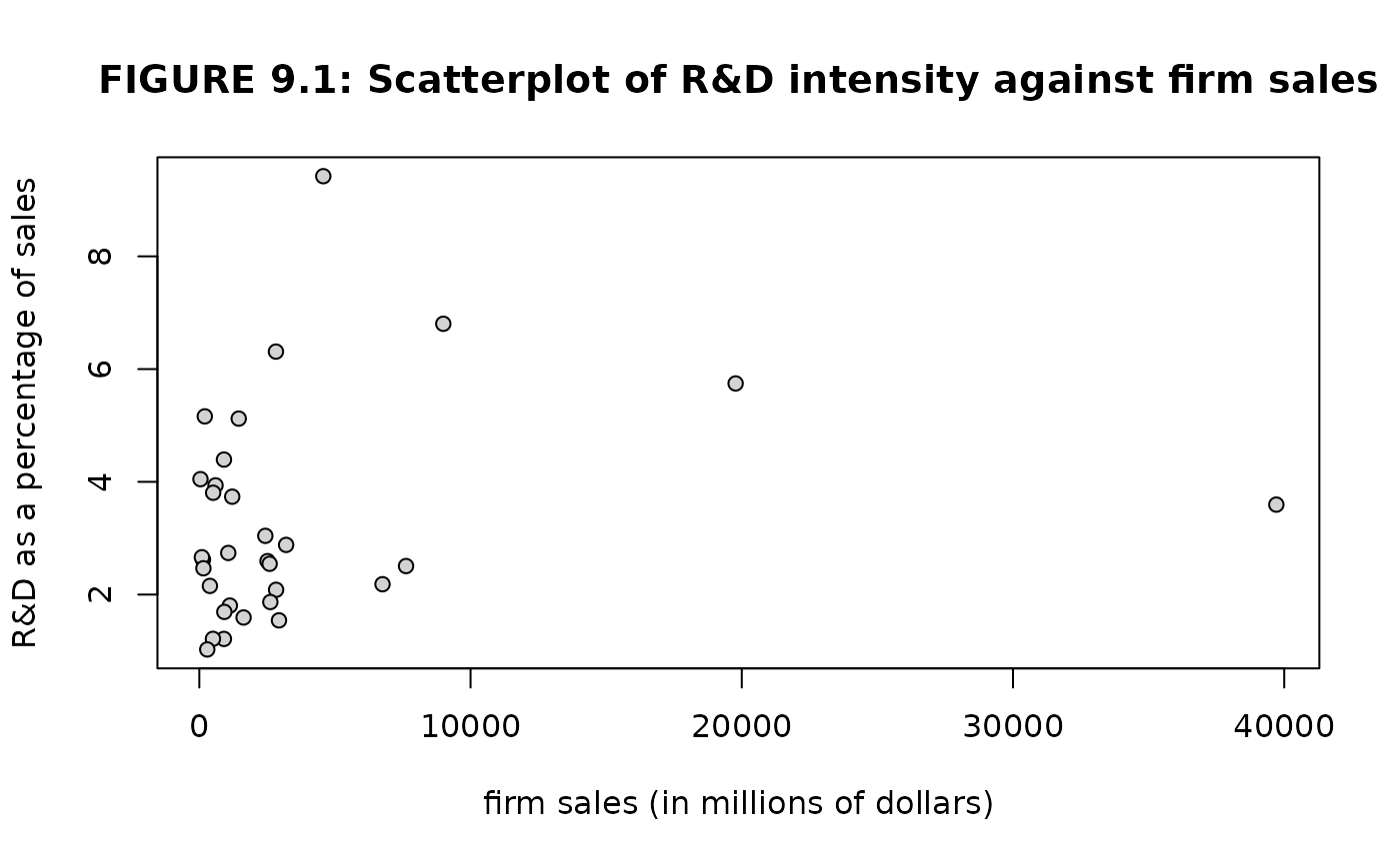
So, we can estimate the model without that data point to gain a better understanding of how sales and profmarg describe rdintens for most firms. We can use the subset argument of the linear model function to indicate that we only want to estimate the model using data that is less than the highest sales.

smallest_rdchem <- lm(rdintens ~ sales + profmarg, data = rdchem, 
                      subset = (sales < max(sales)))

The table below compares the results of both models side by side. By removing the outlier firm, $sales$ become a more significant determination of R&D expenditures.

	Dependent variable:
	rdintens
	(1)	(2)
sales	0.00005 (0.00004)	0.00019** (0.00008)
profmarg	0.04462 (0.04618)	0.04784 (0.04448)
Constant	2.62526*** (0.58553)	2.29685*** (0.59180)
Observations	32	31
R2	0.07612	0.17281
Adjusted R2	0.01240	0.11372
Residual Std. Error	1.86205 (df = 29)	1.79218 (df = 28)
F Statistic	1.19465 (df = 2; 29)	2.92476* (df = 2; 28)
Note:	p<0.1; p<0.05; p<0.01

Chapter 10: Basic Regression Analysis with Time Series Data

Example 10.2: Effects of Inflation and Deficits on Interest Rates

$$\widehat{i3} = \beta_0 + \beta_1inf_t + \beta_2def_t$$ Data from the Economic Report of the President, 2004, Tables B-64, B-73, and B-79.

data("intdef") # load data
# load eXtensible Time Series package.
# xts is excellent for time series plots and 
# properly indexing time series.
library(xts) 
# create xts object from data.frame
# First, index year as yearmon class of monthly data. 
# Note: I add 11/12 to set the month to December, end of year.
index <- zoo::as.yearmon(intdef$year + 11/12)
# Next, create the xts object, ordering by the index above.
intdef.xts <- xts(intdef[ ,-1], order.by = index) 
# extract 3-month Tbill, inflation, and deficit data
intdef.xts <- intdef.xts[ ,c("i3", "inf", "def")] 
# rename with clearer names
colnames(intdef.xts) <- c("Tbill3mo", "cpi", "deficit") 
# plot the object, add a title, and place legend at top left.
plot(x = intdef.xts, 
     main = "Inflation, Deficits, and Interest Rates",
     legend.loc = "topleft")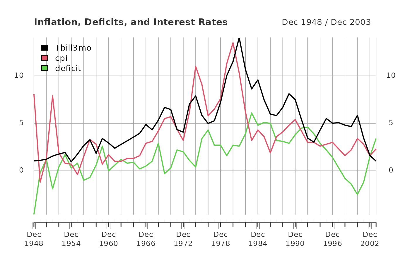

# Run a Linear regression model
tbill_model <- lm(Tbill3mo ~ cpi + deficit, data = intdef.xts)

	Dependent variable:
	Tbill3mo
cpi	0.60587*** (0.08213)
deficit	0.51306*** (0.11838)
Constant	1.73327*** (0.43197)
Observations	56
R2	0.60207
Adjusted R2	0.58705
Residual Std. Error	1.84316 (df = 53)
F Statistic	40.09424*** (df = 2; 53)
Note:	p<0.1; p<0.05; p<0.01

Now lets update the example with current data, pull from the Federal Reserve Economic Research (FRED) using the quantmod package. Other than the convenient API, the package also formats time series data into xts: eXtensible Time Series objects, which add many feature and benefits when working with time series.

# DO NOT RUN
library(quantmod)

# Tbill, 3 month
getSymbols("TB3MS", src = "FRED")
# convert to annual observations and convert index to type `yearmon`.
TB3MS <- to.yearly(TB3MS, OHLC=FALSE, drop.time = TRUE)
index(TB3MS) <- zoo::as.yearmon(index(TB3MS))

# Inflation
getSymbols("FPCPITOTLZGUSA", src = "FRED")
# Convert the index to yearmon and shift FRED's Jan 1st to Dec
index(FPCPITOTLZGUSA) <- zoo::as.yearmon(index(FPCPITOTLZGUSA)) + 11/12
# Rename and update column names
inflation <- FPCPITOTLZGUSA
colnames(inflation) <- "inflation"

## Deficit, percent of GDP: Federal outlays - federal receipts
 # Download outlays
getSymbols("FYFRGDA188S", src = "FRED")
 # Lets move the index from Jan 1st to Dec 30th/31st
index(FYFRGDA188S) <- zoo::as.yearmon(index(FYFRGDA188S)) + 11/12
 # Rename and update column names
outlays <- FYFRGDA188S
colnames(outlays) <- "outlays"

 # Download receipts
getSymbols("FYONGDA188S", src = "FRED")
 # Lets move the index from Jan 1st to Dec 30th/31st
index(FYONGDA188S) <- zoo::as.yearmon(index(FYONGDA188S)) + 11/12
 # Rename and update column names
receipts <- FYONGDA188S
colnames(receipts) <- "receipts"

Now that all data has been downloaded, we can calculate the deficit from the federal outlays and receipts data. Next, we will merge our new deficit variable with inflation and TB3MS variables. As these are all xts times series objects, the merge function will automatically key off each series time date index, insuring integrity and alignment among each observation and its respective date. Additionally, xts provides easy chart construction with its plot method.

# DO NOT RUN
# create deficits from outlays - receipts
# xts objects respect their indexing and outline the future
deficit <- outlays - receipts
colnames(deficit) <- "deficit"

# Merge and remove leading and trailing NAs for a balanced data matrix
intdef_updated <- merge(TB3MS, inflation, deficit)
intdef_updated <- zoo::na.trim(intdef_updated)

#Plot all
plot(intdef_updated, 
     main = "T-bill (3mo rate), inflation, and deficit (% of GDP)",
     legend.loc = "topright",)

Now lets run the model again. Inflation plays a much more prominent role in the 3 month T-bill rate, than the deficit.

# DO NOT RUN
updated_model <- lm(TB3MS ~ inflation + deficit, data = intdef_updated)

Chapter 11: Further Issues in Using OLS with with Time Series Data

Example 11.7: Wages and Productivity

$$\widehat{log(hrwage_t)} = \beta_0 + \beta_1log(outphr_t) + \beta_2t + \mu_t$$ Data from the Economic Report of the President, 1989, Table B-47. The data are for the non-farm business sector.

data("earns")

wage_time <- lm(lhrwage ~ loutphr + t, data = earns)

wage_diff <- lm(diff(lhrwage) ~ diff(loutphr), data = earns)

	Dependent variable:
	lhrwage	diff(lhrwage)
	(1)	(2)
loutphr	1.63964*** (0.09335)
t	-0.01823*** (0.00175)
diff(loutphr)		0.80932*** (0.17345)
Constant	-5.32845*** (0.37445)	-0.00366 (0.00422)
Observations	41	40
R2	0.97122	0.36424
Adjusted R2	0.96971	0.34750
Residual Std. Error (df = 38)	0.02854	0.01695
F Statistic	641.22430*** (df = 2; 38)	21.77054*** (df = 1; 38)
Note:	p<0.1; p<0.05; p<0.01

Chapter 12: Serial Correlation and Heteroskedasticiy in Time Series Regressions

Example 12.8: Heteroskedasticity and the Efficient Markets Hypothesis

These are Wednesday closing prices of value-weighted NYSE average, available in many publications. Wooldridge does not recall the particular source used when he collected these data at MIT, but notes probably the easiest way to get similar data is to go to the NYSE web site, www.nyse.com.

$$return_t = \beta_0 + \beta_1return_{t-1} + \mu_t$$

data("nyse")
?nyse 

return_AR1 <-lm(return ~ return_1, data = nyse)

$$\hat{\mu^2_t} = \beta_0 + \beta_1return_{t-1} + residual_t$$

return_mu <- residuals(return_AR1)
mu2_hat_model <- lm(return_mu^2 ~ return_1, data = return_AR1$model)

	Dependent variable:
	return	return_mu2
	(1)	(2)
return_1	0.05890 (0.03802)	-1.10413*** (0.20140)
Constant	0.17963** (0.08074)	4.65650*** (0.42768)
Observations	689	689
R2	0.00348	0.04191
Adjusted R2	0.00203	0.04052
Residual Std. Error (df = 687)	2.11040	11.17847
F Statistic (df = 1; 687)	2.39946	30.05460***
Note:	p<0.1; p<0.05; p<0.01

Example 12.9: ARCH in Stock Returns

$$\hat{\mu^2_t} = \beta_0 + \hat{\mu^2_{t-1}} + residual_t$$

We still have return_mu in the working environment so we can use it to create $\hat{\mu^2_t}$, (mu2_hat) and $\hat{\mu^2_{t-1}}$ (mu2_hat_1). Notice the use R’s matrix subset operations to perform the lag operation. We drop the first observation of mu2_hat and squared the results. Next, we remove the last observation of mu2_hat_1 using the subtraction operator combined with a call to the NROW function on return_mu. Now, both contain $688$ observations and we can estimate a standard linear model.

mu2_hat  <- return_mu[-1]^2
mu2_hat_1 <- return_mu[-NROW(return_mu)]^2
arch_model <- lm(mu2_hat ~ mu2_hat_1)

	Dependent variable:
	mu2_hat
mu2_hat_1	0.33706*** (0.03595)
Constant	2.94743*** (0.44023)
Observations	688
R2	0.11361
Adjusted R2	0.11231
Residual Std. Error	10.75907 (df = 686)
F Statistic	87.92263*** (df = 1; 686)
Note:	p<0.1; p<0.05; p<0.01

Chapter 13: Pooling Cross Sections across Time: Simple Panel Data Methods

Example 13.7: Effect of Drunk Driving Laws on Traffic Fatalities

Wooldridge collected these data from two sources, the 1992 Statistical Abstract of the United States (Tables 1009, 1012) and A Digest of State Alcohol-Highway Safety Related Legislation, 1985 and 1990, published by the U.S. National Highway Traffic Safety Administration. $$\widehat{\Delta{dthrte}} = \beta_0 + \Delta{open} + \Delta{admin}$$

data("traffic1")
?traffic1

DD_model <- lm(cdthrte ~ copen + cadmn, data = traffic1)

	Dependent variable:
	cdthrte
copen	-0.41968** (0.20559)
cadmn	-0.15060 (0.11682)
Constant	-0.49679*** (0.05243)
Observations	51
R2	0.11867
Adjusted R2	0.08194
Residual Std. Error	0.34350 (df = 48)
F Statistic	3.23144** (df = 2; 48)
Note:	p<0.1; p<0.05; p<0.01

Chapter 18: Advanced Time Series Topics

Example 18.8: FORECASTING THE U.S. UNEMPLOYMENT RATE

Data from Economic Report of the President, 2004, Tables B-42 and B-64.

data("phillips")
?phillips

$$\widehat{unemp_t} = \beta_0 + \beta_1unem_{t-1}$$

Estimate the linear model in the usual way and note the use of the subset argument to define data equal to and before the year 1996.

phillips_train <- subset(phillips, year <= 1996)

unem_AR1 <- lm(unem ~ unem_1, data = phillips_train)

$$\widehat{unemp_t} = \beta_0 + \beta_1unem_{t-1} + \beta_2inf_{t-1}$$

unem_inf_VAR1 <- lm(unem ~ unem_1 + inf_1, data = phillips_train)

	Dependent variable:
	unem
	(1)	(2)
unem_1	0.73235*** (0.09689)	0.64703*** (0.08381)
inf_1		0.18358*** (0.04118)
Constant	1.57174*** (0.57712)	1.30380** (0.48969)
Observations	48	48
R2	0.55397	0.69059
Adjusted R2	0.54427	0.67684
Residual Std. Error	1.04857 (df = 46)	0.88298 (df = 45)
F Statistic	57.13184*** (df = 1; 46)	50.21941*** (df = 2; 45)
Note:	p<0.1; p<0.05; p<0.01

Now, use the subset argument to create our testing data set containing observation after 1996. Next, pass the both the model object and the test set to the predict function for both models. Finally, cbind or “column bind” both forecasts as well as the year and unemployment rate of the test set.

phillips_test <- subset(phillips, year >= 1997)

AR1_forecast <- predict.lm(unem_AR1, newdata = phillips_test)
VAR1_forecast <- predict.lm(unem_inf_VAR1, newdata = phillips_test)

kable(cbind(phillips_test[ ,c("year", "unem")], AR1_forecast, VAR1_forecast))

	year	unem	AR1_forecast	VAR1_forecast
50	1997	4.9	5.526452	5.348468
51	1998	4.5	5.160275	4.896451
52	1999	4.2	4.867333	4.509137
53	2000	4.0	4.647627	4.425175
54	2001	4.8	4.501157	4.516062
55	2002	5.8	5.087040	4.923537
56	2003	6.0	5.819394	5.350271

Appendix

Using R for Introductory Econometrics

This is an excellent open source complimentary text to “Introductory Econometrics” by Jeffrey M. Wooldridge and should be your number one resource. This excerpt from the book’s website:

This book introduces the popular, powerful and free programming language and software package R with a focus on the implementation of standard tools and methods used in econometrics. Unlike other books on similar topics, it does not attempt to provide a self-contained discussion of econometric models and methods. Instead, it builds on the excellent and popular textbook “Introductory Econometrics” by Jeffrey M. Wooldridge.

Heiss, Florian. Using R for Introductory Econometrics. ISBN: 979-8648424364, CreateSpace Independent Publishing Platform, 2020, Dusseldorf, Germany.

url: http://www.urfie.net/.

Applied Econometrics with R

From the publisher’s website:

This is the first book on applied econometrics using the R system for statistical computing and graphics. It presents hands-on examples for a wide range of econometric models, from classical linear regression models for cross-section, time series or panel data and the common non-linear models of microeconometrics such as logit, probit and tobit models, to recent semiparametric extensions. In addition, it provides a chapter on programming, including simulations, optimization, and an introduction to R tools enabling reproducible econometric research. An R package accompanying this book, AER, is available from the Comprehensive R Archive Network (CRAN) at https://CRAN.R-project.org/package=AER.

Kleiber, Christian and Achim Zeileis. Applied Econometrics with R. ISBN 978-0-387-77316-2, Springer-Verlag, 2008, New York. https://link.springer.com/book/10.1007/978-0-387-77318-6

Bibliography

Jeffrey M. Wooldridge (2020). Introductory Econometrics: A Modern Approach, 7th edition. ISBN-13: 978-1-337-55886-0. Mason, Ohio :South-Western Cengage Learning.

Jeffrey A. Ryan and Joshua M. Ulrich (2020). quantmod: Quantitative Financial Modelling Framework. R package version 0.4.18. https://CRAN.R-project.org/package=quantmod

R Core Team (2021). R: A language and environment for statistical computing. R Foundation for Statistical Computing, Vienna, Austria. URL https://www.R-project.org/.

Marek Hlavac (2018). stargazer: Well-Formatted Regression and Summary Statistics Tables. R package version 5.2.2. URL: https://CRAN.R-project.org/package=stargazer

van der Loo M (2020). tinytest “A method for deriving information from running R code.” The R Journal, Accepted for publication. <URL: https://arxiv.org/abs/2002.07472>.

Yihui Xie (2021). knitr: A General-Purpose Package for Dynamic Report Generation in R. R package version 1.33. https://CRAN.R-project.org/package=knitr