Introduction

Download the file 7.R.RData and load it into R using the load function.

data_address <- "https://lagunita.stanford.edu/c4x/HumanitiesSciences/StatLearning/asset/7.R.RData"
download.file(data_address, paste0(getwd(), "/R"))

7.R.R1

Load the data from the file 7.R.RData, and plot it using plot(x,y). What is the slope coefficient in a linear regression of y on x (to within 10%)?

load(path.expand("~/R/StatisticalLearning/data/7R.RData"))
plot(x,y)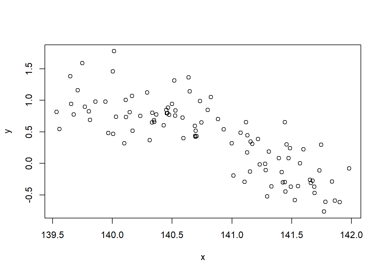

model_71 <- lm(y ~ x)

summary(model_71)

## 
## Call:
## lm(formula = y ~ x)
## 
## Residuals:
##      Min       1Q   Median       3Q      Max 
## -0.71289 -0.26943 -0.02448  0.21068  0.83582 
## 
## Coefficients:
##             Estimate Std. Error t value Pr(>|t|)    
## (Intercept) 95.43627    7.14200   13.36   <2e-16 ***
## x           -0.67483    0.05073  -13.30   <2e-16 ***
## ---
## Signif. codes:  0 '***' 0.001 '**' 0.01 '*' 0.05 '.' 0.1 ' ' 1
## 
## Residual standard error: 0.3376 on 98 degrees of freedom
## Multiple R-squared:  0.6436, Adjusted R-squared:   0.64 
## F-statistic:   177 on 1 and 98 DF,  p-value: < 2.2e-16

7.R.R2

For the model \(y\) ~ \(1 + x + x^2\), what is the coefficient of x (to within 10%)?

model_72 <- lm(y ~ I(x) + I(x^2))

summary(model_72)

## 
## Call:
## lm(formula = y ~ I(x) + I(x^2))
## 
## Residuals:
##      Min       1Q   Median       3Q      Max 
## -0.65698 -0.18190 -0.01938  0.16355  0.86149 
## 
## Coefficients:
##               Estimate Std. Error t value Pr(>|t|)    
## (Intercept) -5.421e+03  1.547e+03  -3.505 0.000692 ***
## I(x)         7.771e+01  2.197e+01   3.536 0.000624 ***
## I(x^2)      -2.784e-01  7.805e-02  -3.567 0.000563 ***
## ---
## Signif. codes:  0 '***' 0.001 '**' 0.01 '*' 0.05 '.' 0.1 ' ' 1
## 
## Residual standard error: 0.3191 on 97 degrees of freedom
## Multiple R-squared:  0.6849, Adjusted R-squared:  0.6784 
## F-statistic: 105.4 on 2 and 97 DF,  p-value: < 2.2e-16