Introduction to RUGtools
Justin M. Shea
June 13th, 2019
Introduction-RUGtools.RmdR User Group Introduction Slides template
This is a traditional ioslides R Markdown template, but modified to contain default content routinely used when introducing Chicago R user group meetups. Slides are useful because they look good and you won’t forget to do important things like thanking the sponsors! Slides can be accessed from within R Studio using the New R Markdown dialog menu, and then selecting From Template. One can also use the draft function, exemplified below.
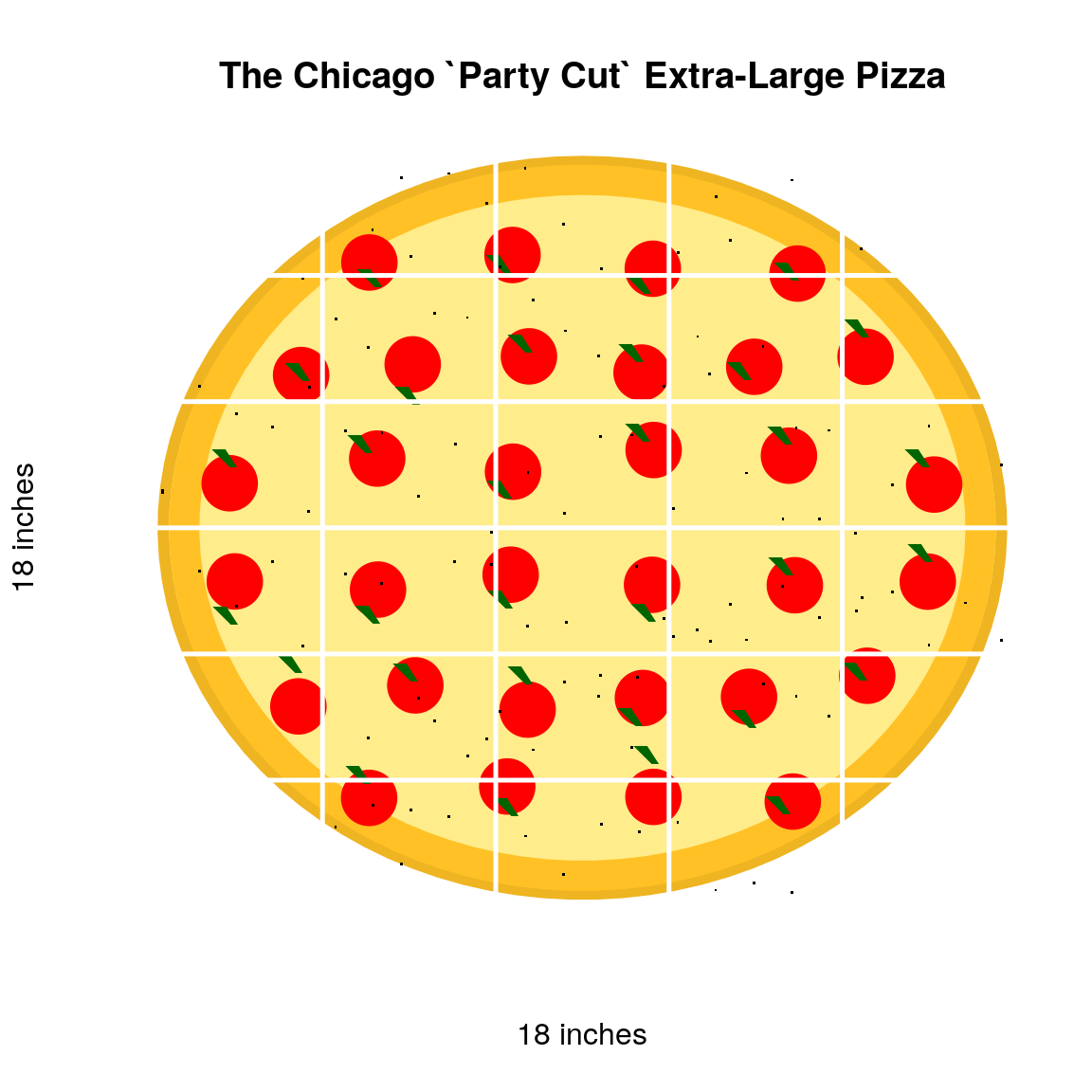
Estimate your pizza order
In Chicago, we think a lot about Pizza. And if one is involved in the local meetup culture, this is doubly so. At a recent meetup group that wasn’t ours, I counted nearly 6 large pizzas left over. Struck by an overwhelming sorrow, I vowed the Chicago R User Group shall never partake in such a tragic waste of resources. With a few data points, one can use the pizza_estimate function to arrive at a more efficient order.
kable( pizza_estimate(registered = 120, pizza_diameter = 18, attend_rate = 0.57,
serving = 2, style = "thin") )| registered | est_attend | eaters_per_pizza | style | pizza_estimate |
|---|---|---|---|---|
| 120 | 69 | 5.342811 | thin | 13 |
Channeling our ever-curious pizza scientist, it turns out the Chicago “party cut” (thin-crust cut into small squares) inherits a few very attractive properties when dividing p pizzas among n guests. Small square pieces allow guests to better estimate pizza consumption, thus decreasing the integer-programming problem exacerbated by large triangular slices. Reducing wasted pizza is not only virtuous, it demonstrates great stewardship of sponsor resources bestowed upon thee.
Data Analysis
Chicago R User Group data is included and downloaded from meetup.com/ChicagoRUG. Personally identifiable information has been removed, data formatted and ready for analysis.
Load the member list data. How many members do we have?
## [1] 3606Lets plot the cumulative membership.
plot(y = member_list$Member.ID, x = member_list$Joined.Group.on, type = "l", lwd=2,
     col = "blue", frame = FALSE, main = "Chicago R User Group members",
     ylab = "Members", xlab = "", ylim = c(0, 4000),
     xlim=c(min(member_list$Joined.Group.on), as.Date("2020-01-01")))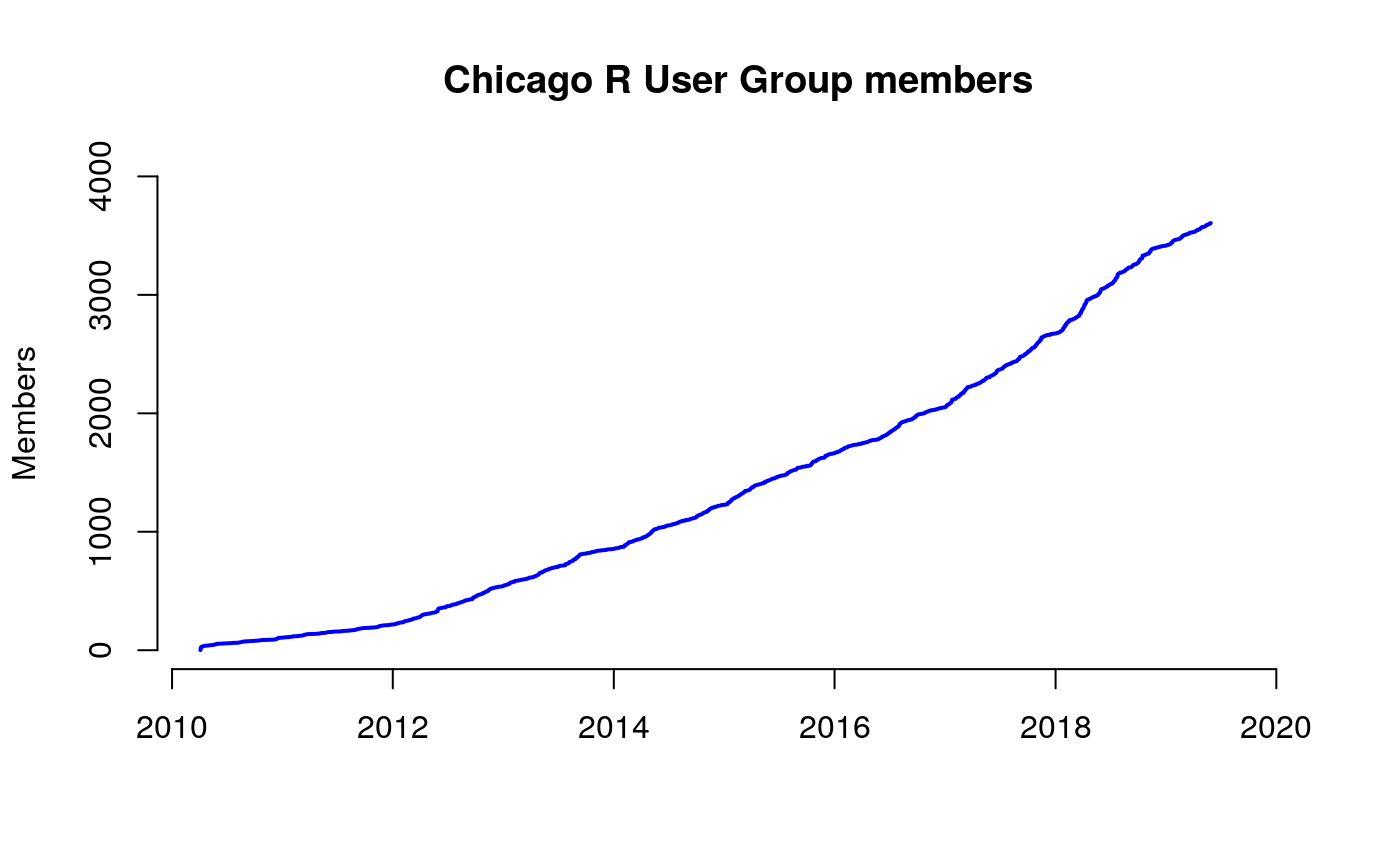
How many members joined since January 2017?
## [1] 1554What percentage of the Chicago R User Group joined since January 2017?
Percentage <- 100 * NROW(subset(member_list, Joined.Group.on > "2017-01-01")) / NROW(member_list)
round(Percentage, 2)
## [1] 43.09How many new members usually join between meetups?
First, get a unique ordered list of Meetup dates
Meetup_dates <- sort(unique(member_list$Last.Attended))

new_members <- subset(member_list, Joined.Group.on > Meetup_dates[NROW(Meetup_dates)])
Then count the number of new members joined between the most recent meetup and the one prior to that.
new_members2 <- subset(member_list, Joined.Group.on <= Meetup_dates[NROW(Meetup_dates)] &
                                    Joined.Group.on > Meetup_dates[NROW(Meetup_dates)-1])

nrow(new_members2)
## [1] 67In danger of repeating the above analysis several times over, we created a function new_mem_counter to count the number of new members joined between meetups for all meetups in the data set.
new_members <- new_mem_counter(member_list)
# drop the last observation, as incomplete data leading up to the coming meetup.
new_members <- new_members[-NROW(new_members),]

kable(head(new_members), align = 'l')| Date | New |
|---|---|
| 2010-05-27 | 0 |
| 2010-08-26 | 20 |
| 2010-10-20 | 10 |
| 2010-12-16 | 15 |
| 2011-03-23 | 34 |
| 2011-06-02 | 17 |
| Date | New | |
|---|---|---|
| 65 | 2018-10-16 | 101 |
| 66 | 2018-11-14 | 52 |
| 67 | 2019-01-23 | 65 |
| 68 | 2019-02-27 | 50 |
| 69 | 2019-03-20 | 19 |
| 70 | 2019-05-15 | 66 |
Which gap between meetups had the most new members?
| Date | New | |
|---|---|---|
| 37 | 2016-06-05 | 157 |
Note the previous meetup was 6 months prior, so likely this was not due to the topic covered.
What is the average number of new members joined between meetups?
## [1] 49.54286Plot the new members data.
   # Create Date Range Index
  Date_Index <- as.numeric(row.names(new_members[new_members$Date > "2010-01-01" & new_members$Date <= Sys.Date(),]))

  # Create x-axis labels, using year-month date format
  x_labels <- format(new_members$Date[Date_Index], "%Y-%m")

  # Plot
  barplot(new_members$New[Date_Index], names.arg = x_labels, main = "CRUG members, joined between meetups",
          ylab = "New Members", xlab = "")
Plot the new members data since 2017.
   # Create Date Range Index
  Date_Index <- as.numeric(row.names(new_members[new_members$Date > "2017-01-01" & new_members$Date <= Sys.Date(),]))

  x_labels <- format(new_members$Date[Date_Index], "%Y-%m")

  # Plot
  barplot(new_members$New[Date_Index], names.arg = x_labels, las=2, main = "CRUG members, joined between meetups",
          ylab = "New Members", xlab = "")
What is the average number of new members joined between meetups since 2017?
## [1] 64.33333Membership as time series
Load and use the xts package.
library(xts)

members_xts <- xts(x = member_list$Member.ID, order.by = member_list$Joined.Group.on)
names(members_xts) <- "useRs"

plot(members_xts, col = "blue", grid.col = "white", main = "Chicago R User Group members by join date")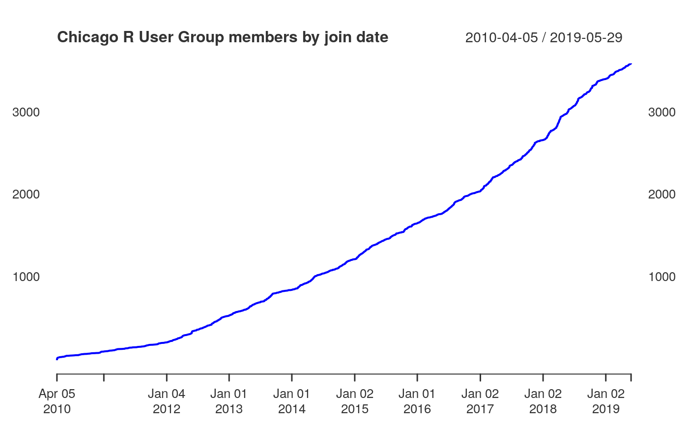
How many members join by month?
members_monthly <- to.monthly(members_xts, OHLC = FALSE)

barplot(diff(members_monthly), col = "lightgrey", main = "Chicago R User Group, new members by month")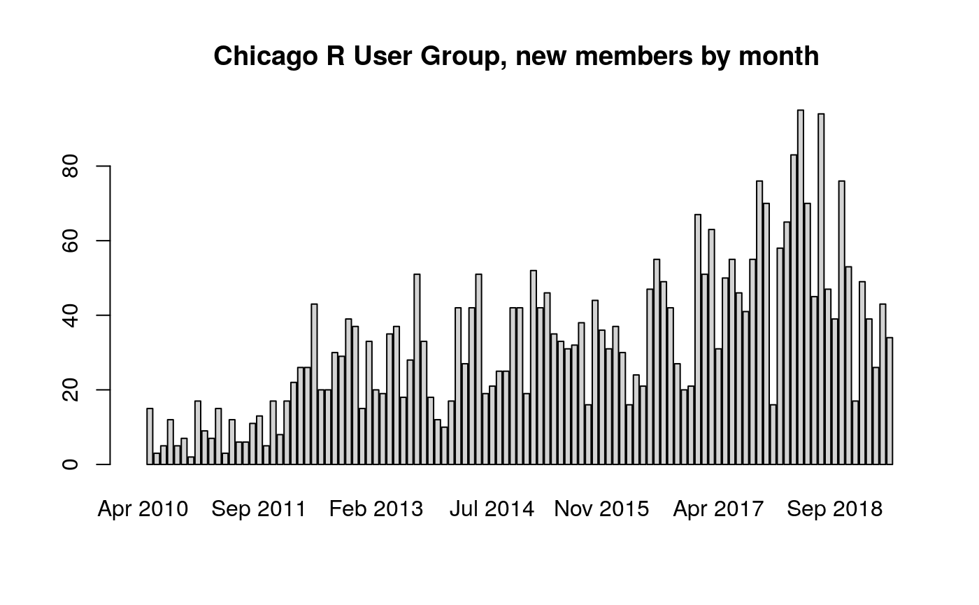
What’s our percentage growth per month?
Omit the first two months growth outliers.
barplot(100*diff(members_monthly)[-c(1,2)]/members_monthly[-c(1,2)], col = "lightgrey",
        main = "CRUG Growth since inception", ylab="Percent")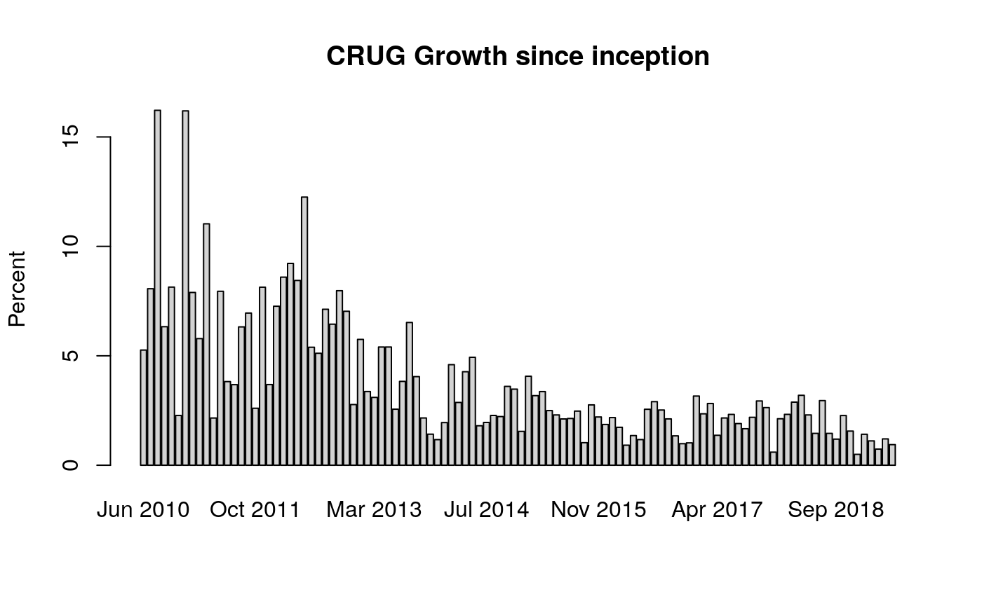
Let’s view the last 4 years.
members_3_years <- 100*diff(members_monthly["2015-05/"]) / members_monthly["2015-05/"]
barplot(members_3_years, col = "lightgrey", main = "CRUG Growth, last 4 years", ylab="Percent")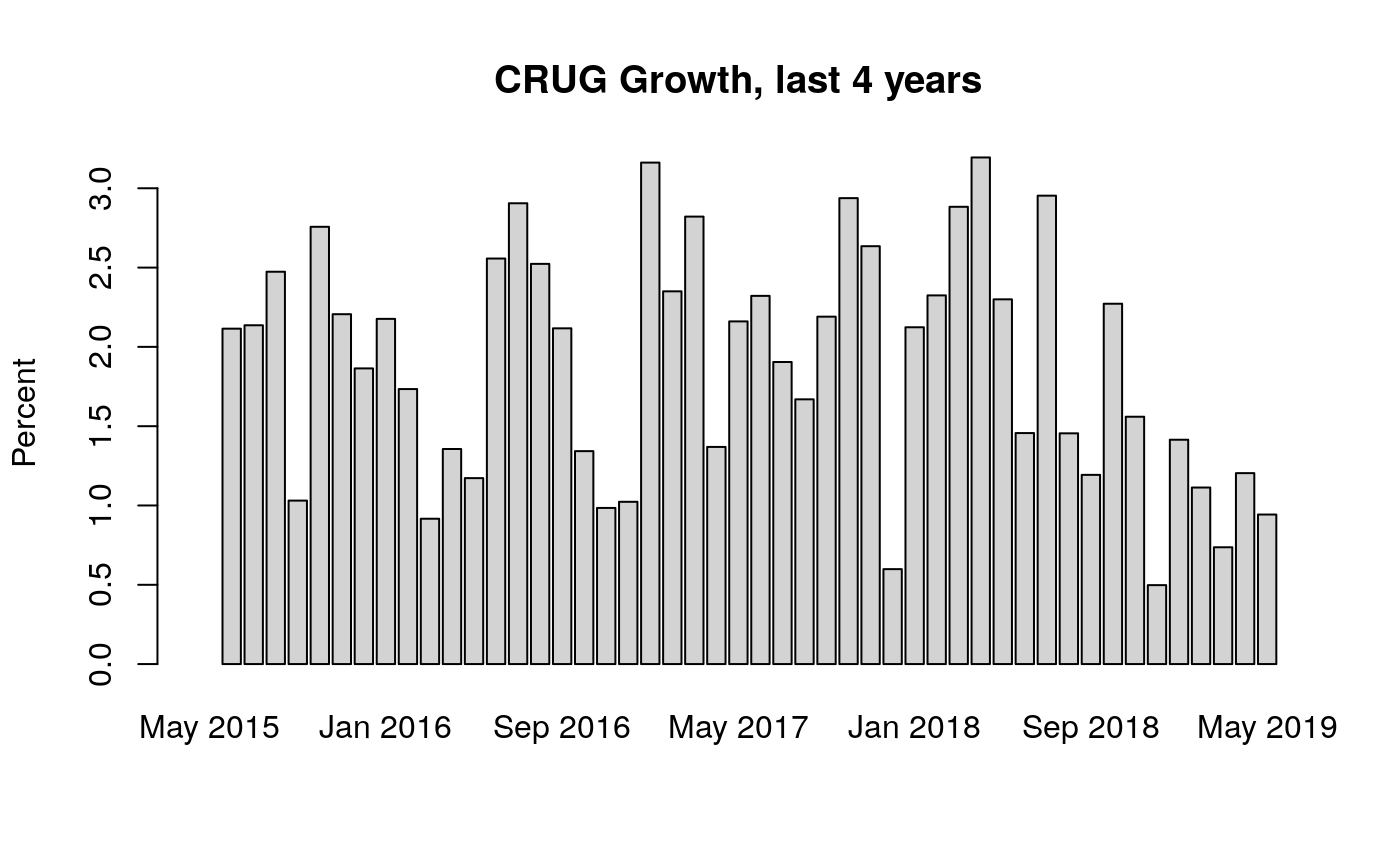
Consider seasonal variation.
month_percent_growth <- c(NA, NA, NA, NA, 100*diff(log(coredata(members_monthly))), NA, NA, NA, NA, NA, NA, NA)
seasonal_matrix <- matrix(month_percent_growth, ncol = 12, byrow = TRUE)
colnames(seasonal_matrix) <- month.abb
rownames(seasonal_matrix) <- 2010:2019
seasonal_matrix <- rbind(seasonal_matrix, Median=round(apply(seasonal_matrix, 2, median, na.rm=TRUE), 2))

kable(seasonal_matrix, digits=2, caption = "Percentage Growth per Month")| Jan | Feb | Mar | Apr | May | Jun | Jul | Aug | Sep | Oct | Nov | Dec | |
|---|---|---|---|---|---|---|---|---|---|---|---|---|
| 2010 | NA | NA | NA | NA | 32.54 | 5.41 | 8.41 | 17.69 | 6.54 | 8.49 | 2.30 | 17.66 |
| 2011 | 8.22 | 5.96 | 11.69 | 2.18 | 8.28 | 3.90 | 3.75 | 6.53 | 7.21 | 2.64 | 8.48 | 3.76 |
| 2012 | 7.54 | 8.99 | 9.67 | 8.82 | 13.07 | 5.54 | 5.25 | 7.39 | 6.66 | 8.31 | 7.29 | 2.81 |
| 2013 | 5.92 | 3.42 | 3.15 | 5.55 | 5.55 | 2.59 | 3.91 | 6.74 | 4.13 | 2.18 | 1.43 | 1.18 |
| 2014 | 1.97 | 4.70 | 2.91 | 4.37 | 5.06 | 1.82 | 1.97 | 2.30 | 2.25 | 3.67 | 3.54 | 1.56 |
| 2015 | 4.15 | 3.23 | 3.42 | 2.53 | 2.33 | 2.14 | 2.16 | 2.51 | 1.04 | 2.80 | 2.23 | 1.88 |
| 2016 | 2.20 | 1.75 | 0.92 | 1.37 | 1.18 | 2.59 | 2.95 | 2.56 | 2.14 | 1.35 | 0.99 | 1.03 |
| 2017 | 3.21 | 2.38 | 2.86 | 1.38 | 2.18 | 2.35 | 1.92 | 1.68 | 2.21 | 2.98 | 2.67 | 0.60 |
| 2018 | 2.15 | 2.35 | 2.93 | 3.25 | 2.33 | 1.47 | 3.00 | 1.47 | 1.20 | 2.30 | 1.57 | 0.50 |
| 2019 | 1.42 | 1.12 | 0.74 | 1.21 | 0.95 | NA | NA | NA | NA | NA | NA | NA |
| Median | 3.21 | 3.23 | 2.93 | 2.53 | 3.69 | 2.59 | 3.00 | 2.56 | 2.25 | 2.80 | 2.30 | 1.56 |
As one of the largest and oldest R user groups in existence, the Chicago R User Group has matured into a comfortable period of value. Growth rates are lower by percentage, but the group continues to serve a steady group of new useRs.